6. Bonus Content - Classifying Office Action Text

So I have obtained prosecution histories for around 100 cases. These are then put through a processing pipeline to extract text sections from the PDF files via the tesseract Optical Character Recognition (OCR) engine.

I have then manually annotated each section to classify it into one of the following classes:

OBJECTION_TYPES = [
    'citation',
    'unity',
    'clarity',
    'added subject matter',
    'conciseness',
    'sufficiency',
    'novelty',
    'inventive step',
    'patentability',
    'other',
    'formalities'
    ]

Now at this stage there are multiple caveats:

The section extraction is not great - the text is quite noisy and it is difficult to always successfully extract the sections correctly. This means there is often section text that mixes different portions of the office action. I have tried to manually clean the worst examples in the data used here. It is a question whether we run a multi-class classification on the whole OCR text or try to split it up. For a test project, the noisy smaller text portions are easier to work with.
The data is fairly limited. We ideally want >10x the data we have. For example, "sufficiency" only has a few examples.

But it may be instructive to have a look at performance on this limited dataset to see whether the automated classification of text has promise.

Loading Data

I manually annotated the data as a spreadsheet. We thus need to load the data from the spreadsheet.

from openpyxl import load_workbook

wb = load_workbook('data_to_label_processed.xlsx')
active_sheet = wb[wb.sheetnames[0]]
read_data = []
for row in active_sheet.rows:
    row_data = []
    for column in row:
        row_data.append(column.value)
    read_data.append(row_data)

print("There are {0} records - each record having {1} fields:\n{2}".format(len(read_data), len(read_data[1]), read_data[1]))

There are 1188 records - each record having 8 fields:
['10850871.4', 'EP', '5ae83cdcab21763a9a6bba7d', datetime.datetime(2017, 2, 21, 0, 0), '1', 'Reference is made to the following document(s); the numbering will be\nadhered to in the rest of the procedure.\n\nD1 WO 03/025775 A1 (WELLOGIX INC [US]) 27 March 2003 (2003-03-27)\n\nD2 us 2001/028364 A1 (FREDELL THOMAS [US] ET AL) 11 October 2001\n(2001-10-11)', 'citation', None]

For our classification example we need a set of tuples ("text", "classification"). We'll add the number to the start of the text.

# Skip first row as that is the header
data = [("{0} {1}".format(r[4], r[5]), r[6]) for r in read_data[1:]]
print(data[0])

('1 Reference is made to the following document(s); the numbering will be\nadhered to in the rest of the procedure.\n\nD1 WO 03/025775 A1 (WELLOGIX INC [US]) 27 March 2003 (2003-03-27)\n\nD2 us 2001/028364 A1 (FREDELL THOMAS [US] ET AL) 11 October 2001\n(2001-10-11)', 'citation')

# Check for blank entries - this screws up the label encoding
[(i, t, c) for i, (t,c) in enumerate(data) if not c]

[]

Transforming the Data

Now we need to convert our text data to a numeric equivalent.

from keras.utils import to_categorical
from sklearn.preprocessing import LabelEncoder

Y_class = [d[1] for d in data]

# encode class values as integers
label_e = LabelEncoder()
label_e.fit(Y_class)
encoded_Y = label_e.transform(Y_class)
# convert integers to dummy variables (i.e. one hot encoded)
Y = to_categorical(encoded_Y)
print("Our classes are now a matrix of {0}".format(Y.shape))
print("Original label: {0}; Converted label: {1}".format(Y_class[0], Y[0]))

Using TensorFlow backend.


Our classes are now a matrix of (1187, 10)
Original label: citation; Converted label: [0. 1. 0. 0. 0. 0. 0. 0. 0. 0.]

label_e.classes_

array(['added subject matter', 'citation', 'clarity', 'formalities',
       'inventive step', 'novelty', 'other', 'patentability',
       'sufficiency', 'unity'], dtype='<U20')

from keras.preprocessing.text import Tokenizer

docs = [d[0] for d in data]

# create the tokenizer
t = Tokenizer(num_words=2500)
# fit the tokenizer on the documents
t.fit_on_texts(docs)

X = t.texts_to_matrix(docs, mode='tfidf')

print("Our data has the following dimensionality: ", X.shape)
print("An example array is: ", X[0][0:100])

Our data has the following dimensionality:  (1187, 2500)
An example array is:  [0.         1.78814384 0.79917757 1.54672314 0.         0.93832662
 0.         0.89437137 1.00441907 0.         0.         0.
 0.         1.29298663 0.         0.         0.         0.
 0.         0.         0.         1.46439595 0.         0.
 0.         0.         0.         0.         0.         0.
 0.         0.         0.         0.         0.         0.
 0.         0.         0.         0.         0.         0.
 0.         0.         0.         0.         0.         0.
 2.06700994 0.         0.         0.         0.         0.
 0.         0.         0.         0.         0.         0.
 2.10873391 0.         0.         0.         0.         0.
 0.         0.         0.         0.         0.         0.
 0.         0.         0.         0.         2.05192351 0.
 0.         0.         0.         0.         0.         0.
 0.         0.         0.         6.36750738 0.         2.38799797
 0.         0.         0.         0.         0.         0.
 0.         0.         0.         0.        ]

import numpy as np
# Convert one hot to target integer
Y_integers = np.argmax(Y, axis=1)

Try Some Classifiers

from sklearn.naive_bayes import MultinomialNB
from sklearn.dummy import DummyClassifier
from sklearn.model_selection import cross_val_score

scores = cross_val_score(DummyClassifier(random_state=5), X, Y_integers, cv=10)
print(
        "Random Classifier has an average classification accuracy of {0:.2f}% ({1:.2f}%)".format(
            scores.mean()*100, 
            scores.std()*100
        )
)

Warning: The least populated class in y has only 9 members, which is too few. The minimum number of members in any class cannot be less than n_splits=10.

Random Classifier has an average classification accuracy of 18.98% (3.46%)

As expected we also have a warning that our "sufficiency" class doesn't have enough data points!

import itertools
import numpy as np
import matplotlib.pyplot as plt

from sklearn.model_selection import train_test_split
from sklearn.metrics import confusion_matrix

def plot_confusion_matrix(cm, classes,
                          normalize=False,
                          title='Confusion matrix',
                          cmap=plt.cm.Blues):
    """
    This function prints and plots the confusion matrix.
    Normalization can be applied by setting `normalize=True`.
    """
    if normalize:
        cm = (cm.astype('float') / cm.sum(axis=1)[:, np.newaxis])*100
        print("Normalized confusion matrix")
    else:
        print('Confusion matrix, without normalization')

    print(cm)

    plt.imshow(cm, interpolation='nearest', cmap=cmap)
    plt.title(title)
    plt.colorbar()
    tick_marks = np.arange(len(classes))
    plt.xticks(tick_marks, classes, rotation=45)
    plt.yticks(tick_marks, classes)

    fmt = '.1f' if normalize else 'd'
    thresh = cm.max() / 2.
    for i, j in itertools.product(range(cm.shape[0]), range(cm.shape[1])):
        plt.text(j, i, format(cm[i, j], fmt),
                 horizontalalignment="center",
                 color="white" if cm[i, j] > thresh else "black")

    plt.tight_layout()
    plt.ylabel('True label')
    plt.xlabel('Predicted label')

import matplotlib
matplotlib.rcParams.update({'font.size': 22})

NBclassifier = MultinomialNB()
scores = cross_val_score(NBclassifier, X, Y_integers, cv=10)
print(
        "Naive Bayes Classifier has an average classification accuracy of {0:.2f} ({1:.2f})".format(
            scores.mean()*100, 
            scores.std()*100
        )
)

Warning: The least populated class in y has only 9 members, which is too few. The minimum number of members in any class cannot be less than n_splits=10.
  % (min_groups, self.n_splits)), Warning)


Naive Bayes Classifier has an average classification accuracy of 63.08 (4.88)

This seems suprisingly similar to our previous task, where we had a classification accuracy of around 60%.

Let's have a closer look at how the classifier is being applied.

X_train, X_test, y_train, y_test = train_test_split(X, Y_integers, random_state=0)

NB_y_pred = NBclassifier.fit(X_train, y_train).predict(X_test)
NB_cnf_matrix = confusion_matrix(y_test, NB_y_pred)
np.set_printoptions(precision=2)

plt.figure(figsize=(20, 20))
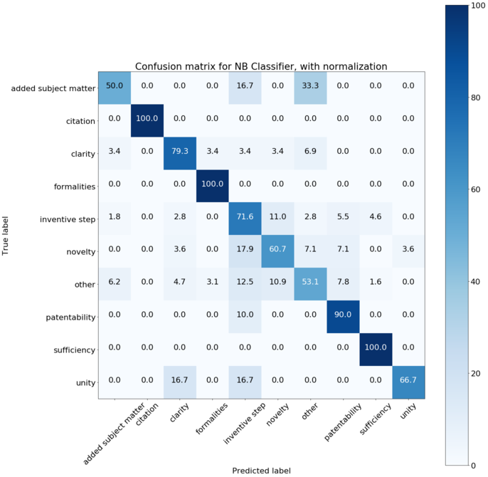
plot_confusion_matrix(NB_cnf_matrix, classes=label_e.classes_, normalize=True,
                      title='Confusion matrix for NB Classifier, with normalization')

plt.show()

Normalized confusion matrix
[[ 50.     0.     0.     0.    16.67   0.    33.33   0.     0.     0.  ]
 [  0.   100.     0.     0.     0.     0.     0.     0.     0.     0.  ]
 [  3.45   0.    79.31   3.45   3.45   3.45   6.9    0.     0.     0.  ]
 [  0.     0.     0.   100.     0.     0.     0.     0.     0.     0.  ]
 [  1.83   0.     2.75   0.    71.56  11.01   2.75   5.5    4.59   0.  ]
 [  0.     0.     3.57   0.    17.86  60.71   7.14   7.14   0.     3.57]
 [  6.25   0.     4.69   3.12  12.5   10.94  53.12   7.81   1.56   0.  ]
 [  0.     0.     0.     0.    10.     0.     0.    90.     0.     0.  ]
 [  0.     0.     0.     0.     0.     0.     0.     0.   100.     0.  ]
 [  0.     0.    16.67   0.    16.67   0.     0.     0.     0.    66.67]]

png

# Lets also try the Multi-layer Perceptron
from sklearn.neural_network import MLPClassifier

MLPclassifier = MLPClassifier()
scores = cross_val_score(MLPclassifier, X, Y_integers, cv=10)
print(
        "MLP Classifier has an average classification accuracy of {0:.2f} ({1:.2f})".format(
            scores.mean()*100, 
            scores.std()*100
        )
)

X_train, X_test, y_train, y_test = train_test_split(X, Y_integers, random_state=0)

MLP_y_pred = MLPclassifier.fit(X_train, y_train).predict(X_test)
MLP_cnf_matrix = confusion_matrix(y_test, MLP_y_pred)
np.set_printoptions(precision=2)

plt.figure(figsize=(20, 20))
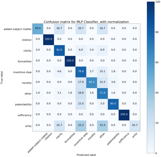
plot_confusion_matrix(MLP_cnf_matrix, classes=label_e.classes_, normalize=True,
                      title='Confusion matrix for MLP Classifier, with normalization')

plt.show()

MLP Classifier has an average classification accuracy of 70.70 (4.68)
Normalized confusion matrix
[[ 50.     0.    16.67   0.    16.67   0.    16.67   0.     0.     0.  ]
 [  0.   100.     0.     0.     0.     0.     0.     0.     0.     0.  ]
 [  0.     0.    82.76   0.     6.9    3.45   6.9    0.     0.     0.  ]
 [  0.     0.     0.   100.     0.     0.     0.     0.     0.     0.  ]
 [  0.     0.     4.59   0.    79.82   3.67  10.09   1.83   0.     0.  ]
 [  0.     0.     0.     0.    17.86  64.29  14.29   3.57   0.     0.  ]
 [  1.56   0.     3.12   1.56  18.75   1.56  71.88   1.56   0.     0.  ]
 [  0.     0.     0.     0.    15.     0.     5.    80.     0.     0.  ]
 [  0.     0.     0.     0.     0.     0.     0.     0.   100.     0.  ]
 [  0.     0.    16.67   0.    33.33   0.    33.33   0.     0.    16.67]]

png

Comments on Results

These are fairly good results out-of-the-box.

I think the main improvements would come from:

cleaner data;
more data;
more consistent labelling.

This also does not take account of the fact that objections are often presented in numbered lists with a hierarchical structure. We can use this as a form of ensemble classifier.