5. Classifying Claims - Reporting Results
Here we will look at what we have learnt during our project to classify patent claims. The aim of doing this is to consolidate what we have learnt, and practice a methodology for presenting our results.
The post here suggests the following structure for reporting our results:
- Context - Define and describe why we are undertaking the project;
- Problem - Describe the problem we are looking to solve;
- Solution - Describe the solution our results suggest;
- Findings - Present our results;
- Limitations - Present the limitations we uncovered; and
- Conclusions - Revisit and summarise the context, problem and solution (or why, question and answer)
We will look at these one by one.
1. Context
As described in our first post, the project was undertaken to practice applying a methodical approach to real-world patent data.
Within the world of patent law, we have sets of patent claims, which set out the scope of legal protection. These claims, as they are contained in a patent application, are assigned a patent classification, which is a hierarchical code that categorises the subject-matter of the claims.
Patent specifications are published and made available for download in bulk. This provides large labelled datasets we can use to practice supervised machine learning. In particular, we can extract a main independent claim and an International Patent Classification (IPC) code as data for machine learning algorithms. To simplify things, we can start with the first letter of the IPC code, which assigns each patent application to one of eight classes.
2. Problem
The problem we are looking to solve is to develop a machine learning algorithm that, given the text of a patent claim, can predict the first letter of the IPC code, i.e. the first level of subject matter classification.
3. Solution
Our results indicate that one of a non-linear Support Vector Machine (SVM), a multi-layer perceptron (MLP) or a Naive Bayes classifier would be the best at performing this task.
For a production solution, it appears preferable to use a Naive Bayes classifier despite the SVM and MLP outperforming this classifier by 2-3%. This is because the Naive Bayes classifier is much more efficient: it is the quickest of the three to train and does not require a large number of parameters. It also has good characteristics, such as performing better at classifying certain classes than the MLP.
From our results it does not seem possible to implement an accurate classifier for this problem. The best solutions return an accuracy of around 60%. While better than chance given the proportions of the data (~20%) this is still not necessarily high enough to confidently apply a classifier in a processing pipeline, e.g. to differentially process the text of the patent claim.
It would, though, appear possible to provide probabilities for classes that could support human decision making.
4. Findings
Our finding will be split into three sections: 1. Findings regarding the nature of the problem and the data; 2. Findings regarding suitable machine learning algorithms; and 3. Findings regarding specific algorithms.
4.1 Findings regarding the nature of the problem and the data
A general finding was that changes in algorithms, parameters, and model archectures only led to small improvements in accuracy (e.g. often along the lines of 1-2%). Generally, the best classification accuracy was fixed at around 60%.
Changing the form of the data had suprisingly little effect.
Term Frequency - Inverse Document Frequency (TD-IDF) was the best metric for generating a bag of words. However, using word presence (i.e. a binary variable) or word count only reduced classification accuracy by 1-2%. This improvement is close to the bounds of natural variance. As such, a Naive Bayes implementation that uses a binary count could be used if processing resources were limited (e.g. within embedded systems). It should be noted that normalising by the sequence length appeared to corrupt Naive Bayes classification.
I imagined that increasing our number of data samples would provide a reasonably large improvement. However, this was not the case - nearly doubling our number of data samples again only provided a 1-2% increase. This improvement is again close to the bounds of natural variance. This suggests that our low accuracy value may be due to the nature of the classification distributions, e.g. it may be dragged down by poor performance on infrequent classes. This is also consistent with the reasonably good performance of the Naive Bayes classifier below.
Similarly, doubling our vocabulary did not have a significant effect on performance, again only increasing accuracy by 1-2%. This indicates that a production system could trade-off accuracy for vocabulary size.
As the TD-IDF metric is already normalised, subtracting the mean and dividing by the variance did not improve performance.
4.2 Findings regarding suitable machine learning algorithms
Spot Check Results
The results of our spot-checks were as follows:
| Classifer | Accuracy | SD |
|---|---|---|
| Non-Linear Support Vector Machine | 62.52 % | 0.80 % |
| MultiLayer Perceptron | 61.20 % | 0.54 % |
| Naive Bayes | 58.90 % | 1.12 % |
| Stochastic Gradient Descent | 56.79 % | 0.75 % |
| Random Forest | 50.01 % | 1.17 % |
| Decision Trees | 47.33 % | 0.52 % |
| Ada Boost | 34.34 % | 1.31 % |
| kNearest Neighbours | 30.15 % | 2.74 % |
| Random Choice | 20.14 % | 0.13 % |
Here we see that our best performing algorithm is the non-linear Support Vector Machine (SVM). SVMs are known to work well on sparse data of high dimensionality. This is the case for us and our results support that finding.
Tree and cluster based methods generally do not perform as well.
However, the training time for the non-linear SVM in scikit-learn (based on libsvm) is very long, much longer than either the MLP or the Naive Bayes classifier. The Naive Bayes classifier is one of the quickest, taking only a few seconds, compared to tens of minutes for the MLP and up to an hour for the SVM.
Comparing Predictions
It was interesting to compare how our Naive Bayes and MLP classifiers were predicting categories.
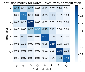
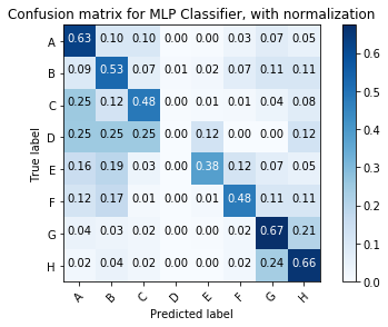
The Naive Bayes classifier struggled on class A - often confusing it with class C. However, it out-performs the MLP classifier on classes C, E, F and G - a majority of the classes.
The MLP classifier obtains a higher classification accuracy by outperforming on classes A and H. Indeed it looks like the misclassification of class A by the Naive Bayes classifier was the main reason for it having an overal accuracy below the MLP.
This is one reason why the Naives Bayes classifier may actually be better in production despite having a headline accuracy below the MLP.
It was disappointing to see that an ensemble classifier did not seem to capitalise on the relative strengths of both classifiers, at least in terms of overall classification accuracy.
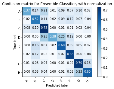
The Naive Bayes brings down the performance of the ensemble classifier for classes A and H, despite increasing the accuracy for the other classes. This suggests that the Naive Bayes classifiers may be assigning fairly high incorrect probabilities for classes A and H, such that a hard or soft vote still goes with the missclassification.
Ensemble classifiers appear a fruitful area for further investigation. For example, it may be that be adjusting the weightings of the ensemble we can avoid the degnerative performance for classes A and H.
4.3 Findings regarding specific algorithms
While the non-linear SVM provided the best performance, it's long training time made it difficult to experiment with. The Naive Bayes classifier has only one tuneable parameter (alpha relating to a level of smoothing). Adjusting this parameter had no real significant affect. Attention was thus focussed on the MLP classifer. To have access to more aspects of configuration we moved to use Keras.
Overfitting
A key finding in this project was the importance of regularisation to avoid overfitting.
Our simple one layer neural network suffered greatly from overfitting on the data.
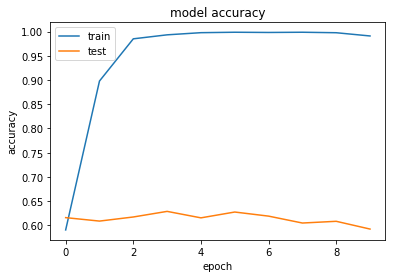
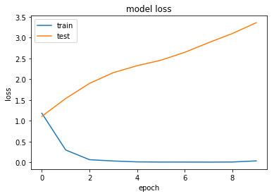
As can be seen in these graphs, within a few epochs our network has a near 100% accuracy as it learns to overfit on the supplied data. Considering that we have 10,000 data samples and, due to the high dimensionality input, our model has 2.5 million parameters, it is easy to see how overfitting could occur - i.e. there are many more parameters than samples so our network can simply learn to memorise each sample.
Overfitting leads to poor performance on validation datasets, i.e. data that is not used to train the neural network. This is most visible in the graph of model loss: while model loss reduces during training for the training data it increases for the test data set, i.e. we perform worse on our test data as our model overfits on our training data.
Two techniques are recommended for overfitting: Dropout and Regularisation. In our case it turned out that Regularisation was more effective, and that a combination of moderate amounts of both Dropout and Regularisation acted to align training and test performance. For example L2 regularisation with a lambda value of 0.05 and Dropout between layers of around 0.2-0.25 worked well.
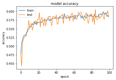
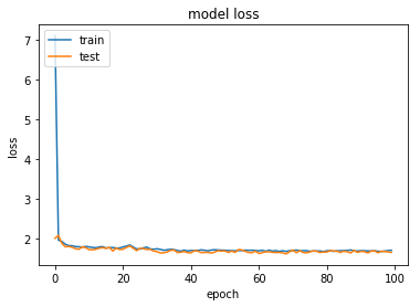
However, even in this case, performance quickly saturates and additional trainings does not do much to increase our accuracy or reduce our loss.
This is consistent with our other results - it suggests that there are certain easily discernable rules for work for 60-80% of class classifications, but that beyond that there are no absolute rules and that certain claims cannot be predictable assigned a class.
Architectures
Moving to deeper and more complex neural network did not significantly improve accuracy. This is an important lesson - there are many different possible architectures we can explore, but ultimately we are dependent on the form of our data.
5. Limitations
There seemed to be a natural limit of around 60% to classifier performance. Here are some ideas for why this may be:
- The claims do not contain enough information. This may especially be the case for particularly broad claims. We need to also look at the text of the detailed description.
- A number of different classifications may be assigned to a patent application. For example, often claims may be classified in both categories G and H. As such the models may be accurate predicting another of the classifications but incorrectly predicting the chosen single category.
- Classifications may be assigned by human beings who are not necessarily consistent. Hence, there may be contradictions in our data.
A number of other limitations were uncovered:
- Computing resources limited the effectiveness of our most accurate classifier.
- Overfitting limited the performance of our neural network models - this was partially mitigated using Dropout and regularisation.
- The compressed XML archives of patent data make it difficult to quickly access large amounts of data - when trying to process 20,000 patent documents, we had errors after processing 19,000. It may be that there are other datasets we can use, such as Google's BigQuery or other downloadable preprocessed sets of claim-classification pairs.
6. Conclusions
So, how best to assign a Section to a patent claim?
It turns out that a Naive Bayes classifier is a good all-round solution. I would select this for any production system. Although SVM and neural network classifiers showed slightly better performance, as measured by overall classification accuracy, the out-of-the-box quick performance of the Naive Bayes classifier, and it's reasonable strengths on individual classes, makes me believe that this is a better solution.
Even with advanced techniques overall classification accuracy was limited to around 60%. This is still better than 20% if chosen at random. However, it suggests that we cannot implement a deterministic system that makes decisions based on programmatically assigned Sections. We may thus need to shift our perspective, e.g. could we show suggested Sections, together with probabilities to help human decision making, or offer a "confirm Section" option that allows the over-riding of the missclassification of certain Sections.