4. Classifying Claims - Improving Results

At this stage, we will look at taking a few of our best-performing algorithms from our previous post and attempting to increase performance.

As you may remember, the best-performing algorithms were:

Naive Bayes - an accuracy of 58.90% (1.12% variance);
SVM with non-linear kernel - an accuracy of 62.52% (0.80% variance); and
Multilayer neural networks - an accuracy of 61.20% (0.54% variance).

Ths posts here and here offer some suggestions for how to increase performance:

Improve Performance With Data.
Improve Performance With Algorithms.
Improve Performance With Algorithm Tuning.
Improve Performance With Ensembles.

We should also look at the time required to train our models. If a model is 10x faster to train, it may be preferable to another model with greater accuracy.

Load the Data

import pickle
with open("encoded_data.pkl", "rb") as f:
    print("Loading data")
    X, Y = pickle.load(f)
    print("{0} claims and {1} classifications loaded".format(len(X), len(Y)))

Loading data
11238 claims and 11238 classifications loaded

import numpy as np
# Convert one hot to target integer
Y_integers = np.argmax(Y, axis=1)

Naive Bayes to Start

It turns out that there are not too many parameters we can vary for a Naive Bayes classifier. In fact, in scikit-learn there is only one tuneable parameter - alpha - that sets an amount of additive smoothing (see the documentation here.

The smoothing is set to 1.0 as a default. Let's have a look at performance if we turn this off by setting the alpha parameter to 0.

from sklearn.model_selection import cross_val_score
from sklearn.naive_bayes import MultinomialNB

scores = cross_val_score(MultinomialNB(alpha=1.0e-3), X, Y_integers, cv=5)

print(
        "NB with alpha = 0 has an average classification accuracy of {0:.2f} ({1:.2f})".format(
            scores.mean()*100, 
            scores.std()*100
        )    
)

NB with alpha = 0 has an average classification accuracy of 58.94 (0.43)

As we can see changing this parameter doesn't seem to have that much effect.

Improving Performance with Algorithms

Now, scikit-learn provides a rather simple multi-layer neural network implementation. To improve performance we can experiment with more advanced neural network architectures.

Questions we can ask include: - Does changing the number of hidden layers increase performance? - Does using Dropout increase performance? - Does changing the dimensionality of our hidden layers increase performance?

Keras is an excellent library for experimenting with deep learning models. We will play around using that. This post here explains how we can perform k-fold validation with keras models.

input_dim = X.shape[1]
print("Our input dimension for our claim representation is {0}".format(input_dim))

no_classes = Y.shape[1]
print("Our output dimension is {0}".format(no_classes))

Our input dimension for our claim representation is 5000
Our output dimension is 8

Keras Model

Before attempting cross-validation, let's build and explore a Keras model.

This post here provides help for obtaining training metrics as Keras callback data and plotting those metrics.

from keras.models import Sequential
from keras.layers import Dense, Activation, Dropout
import matplotlib.pyplot as plt

def keras_model():
    # create model
    model = Sequential()
    model.add(Dense(500, input_dim=input_dim, activation='relu'))
    model.add(Dense(no_classes, activation='softmax'))
    # Compile model
    model.compile(loss='categorical_crossentropy', optimizer='adam', metrics=['accuracy'])
    return model

model = keras_model()
model.summary()
history = model.fit(X, Y, validation_split=0.2, epochs=10, batch_size=5, verbose=1)

# list all data in history
print(history.history.keys())
# summarize history for accuracy
plt.plot(history.history['acc'])
plt.plot(history.history['val_acc'])
plt.title('model accuracy')
plt.ylabel('accuracy')
plt.xlabel('epoch')
plt.legend(['train', 'test'], loc='upper left')
plt.show()
# summarize history for loss
plt.plot(history.history['loss'])
plt.plot(history.history['val_loss'])
plt.title('model loss')
plt.ylabel('loss')
plt.xlabel('epoch')
plt.legend(['train', 'test'], loc='upper left')
plt.show()

_________________________________________________________________
Layer (type)                 Output Shape              Param #   
=================================================================
dense_9 (Dense)              (None, 500)               2500500   
_________________________________________________________________
dense_10 (Dense)             (None, 8)                 4008      
=================================================================
Total params: 2,504,508
Trainable params: 2,504,508
Non-trainable params: 0
_________________________________________________________________
Train on 8990 samples, validate on 2248 samples
Epoch 1/10
8990/8990 [==============================] - 298s - loss: 1.1831 - acc: 0.5908 - val_loss: 1.1081 - val_acc: 0.6161
Epoch 2/10
8990/8990 [==============================] - 297s - loss: 0.3009 - acc: 0.8979 - val_loss: 1.5360 - val_acc: 0.6090
Epoch 3/10
8990/8990 [==============================] - 294s - loss: 0.0672 - acc: 0.9850 - val_loss: 1.8990 - val_acc: 0.6174
Epoch 4/10
8990/8990 [==============================] - 298s - loss: 0.0364 - acc: 0.9932 - val_loss: 2.1578 - val_acc: 0.6290
Epoch 5/10
8990/8990 [==============================] - 307s - loss: 0.0150 - acc: 0.9977 - val_loss: 2.3248 - val_acc: 0.6157
Epoch 6/10
8990/8990 [==============================] - 311s - loss: 0.0105 - acc: 0.9986 - val_loss: 2.4560 - val_acc: 0.6277
Epoch 7/10
8990/8990 [==============================] - 307s - loss: 0.0106 - acc: 0.9981 - val_loss: 2.6464 - val_acc: 0.6192
Epoch 8/10
8990/8990 [==============================] - 308s - loss: 0.0095 - acc: 0.9986 - val_loss: 2.8779 - val_acc: 0.6050
Epoch 9/10
8990/8990 [==============================] - 300s - loss: 0.0117 - acc: 0.9976 - val_loss: 3.0982 - val_acc: 0.6085
Epoch 10/10
8990/8990 [==============================] - 286s - loss: 0.0386 - acc: 0.9909 - val_loss: 3.3565 - val_acc: 0.5925
dict_keys(['val_acc', 'acc', 'loss', 'val_loss'])

png

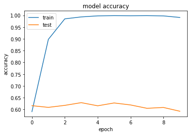
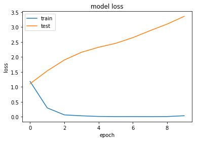
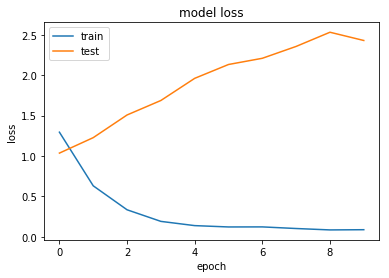
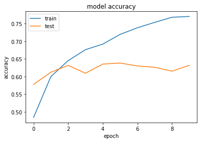
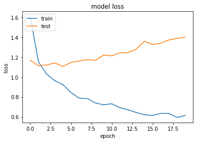
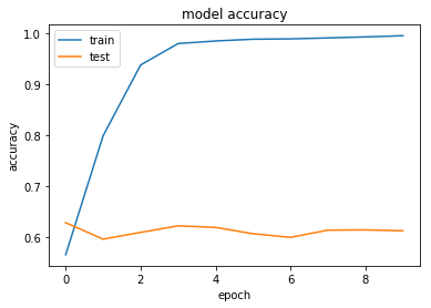
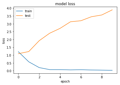
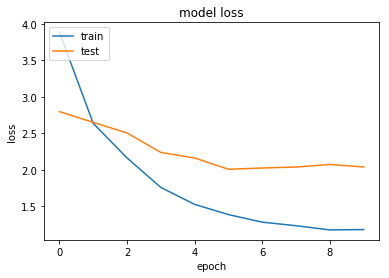
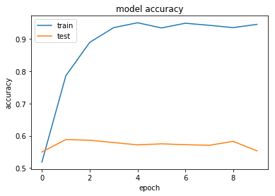
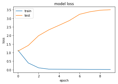
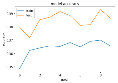
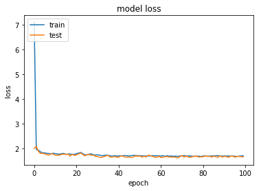
Overfitting

Looking at this first set of results we can see that our neural network quickly overfits the data, while the test performance stays reasonably constant.

One way to reduce overfitting is to apply Dropout. Let's try that now.

from keras.layers import Dropout

def keras_dropout_model():
    # create model
    model = Sequential()
    model.add(Dropout(0.2, input_shape=(input_dim,)))
    model.add(Dense(500, activation='relu'))
    model.add(Dropout(0.2))
    model.add(Dense(no_classes, activation='softmax'))
    # Compile model
    model.compile(loss='categorical_crossentropy', optimizer='adam', metrics=['accuracy'])
    return model

model = keras_dropout_model()
model.summary()
history = model.fit(X, Y, validation_split=0.2, epochs=10, batch_size=5, verbose=1)

# list all data in history
print(history.history.keys())
# summarize history for accuracy
plt.plot(history.history['acc'])
plt.plot(history.history['val_acc'])
plt.title('model accuracy')
plt.ylabel('accuracy')
plt.xlabel('epoch')
plt.legend(['train', 'test'], loc='upper left')
plt.show()
# summarize history for loss
plt.plot(history.history['loss'])
plt.plot(history.history['val_loss'])
plt.title('model loss')
plt.ylabel('loss')
plt.xlabel('epoch')
plt.legend(['train', 'test'], loc='upper left')
plt.show()

_________________________________________________________________
Layer (type)                 Output Shape              Param #   
=================================================================
dropout_1 (Dropout)          (None, 5000)              0         
_________________________________________________________________
dense_11 (Dense)             (None, 500)               2500500   
_________________________________________________________________
dropout_2 (Dropout)          (None, 500)               0         
_________________________________________________________________
dense_12 (Dense)             (None, 8)                 4008      
=================================================================
Total params: 2,504,508
Trainable params: 2,504,508
Non-trainable params: 0
_________________________________________________________________
Train on 8990 samples, validate on 2248 samples
Epoch 1/10
8990/8990 [==============================] - 297s - loss: 1.2949 - acc: 0.5539 - val_loss: 1.0363 - val_acc: 0.6326
Epoch 2/10
8990/8990 [==============================] - 277s - loss: 0.6315 - acc: 0.7833 - val_loss: 1.2275 - val_acc: 0.6174
Epoch 3/10
8990/8990 [==============================] - 268s - loss: 0.3351 - acc: 0.8899 - val_loss: 1.5079 - val_acc: 0.6125
Epoch 4/10
8990/8990 [==============================] - 285s - loss: 0.1916 - acc: 0.9408 - val_loss: 1.6871 - val_acc: 0.6005
Epoch 5/10
8990/8990 [==============================] - 288s - loss: 0.1392 - acc: 0.9590 - val_loss: 1.9611 - val_acc: 0.6143
Epoch 6/10
8990/8990 [==============================] - 272s - loss: 0.1226 - acc: 0.9648 - val_loss: 2.1324 - val_acc: 0.6036
Epoch 7/10
8990/8990 [==============================] - 272s - loss: 0.1233 - acc: 0.9675 - val_loss: 2.2092 - val_acc: 0.6201
Epoch 8/10
8990/8990 [==============================] - 271s - loss: 0.1033 - acc: 0.9730 - val_loss: 2.3560 - val_acc: 0.6170
Epoch 9/10
8990/8990 [==============================] - 273s - loss: 0.0860 - acc: 0.9770 - val_loss: 2.5313 - val_acc: 0.6072
Epoch 10/10
8990/8990 [==============================] - 273s - loss: 0.0886 - acc: 0.9772 - val_loss: 2.4294 - val_acc: 0.6281
dict_keys(['val_acc', 'acc', 'loss', 'val_loss'])

png

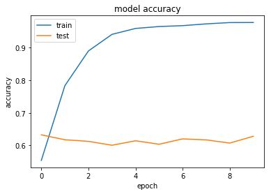
Now let's try with a more aggressive level of Dropout.

from keras.layers import Dropout

def keras_dropout_model():
    # create model
    model = Sequential()
    model.add(Dropout(0.5, input_shape=(input_dim,)))
    model.add(Dense(500, activation='relu'))
    model.add(Dropout(0.5))
    model.add(Dense(no_classes, activation='softmax'))
    # Compile model
    model.compile(loss='categorical_crossentropy', optimizer='adam', metrics=['accuracy'])
    return model

model = keras_dropout_model()
model.summary()
history = model.fit(X, Y, validation_split=0.2, epochs=10, batch_size=5, verbose=1)

# list all data in history
print(history.history.keys())
# summarize history for accuracy
plt.plot(history.history['acc'])
plt.plot(history.history['val_acc'])
plt.title('model accuracy')
plt.ylabel('accuracy')
plt.xlabel('epoch')
plt.legend(['train', 'test'], loc='upper left')
plt.show()
# summarize history for loss
plt.plot(history.history['loss'])
plt.plot(history.history['val_loss'])
plt.title('model loss')
plt.ylabel('loss')
plt.xlabel('epoch')
plt.legend(['train', 'test'], loc='upper left')
plt.show()

_________________________________________________________________
Layer (type)                 Output Shape              Param #   
=================================================================
dropout_3 (Dropout)          (None, 5000)              0         
_________________________________________________________________
dense_13 (Dense)             (None, 500)               2500500   
_________________________________________________________________
dropout_4 (Dropout)          (None, 500)               0         
_________________________________________________________________
dense_14 (Dense)             (None, 8)                 4008      
=================================================================
Total params: 2,504,508
Trainable params: 2,504,508
Non-trainable params: 0
_________________________________________________________________
Train on 8990 samples, validate on 2248 samples
Epoch 1/10
8990/8990 [==============================] - 289s - loss: 1.5896 - acc: 0.4839 - val_loss: 1.1905 - val_acc: 0.5778
Epoch 2/10
8990/8990 [==============================] - 288s - loss: 1.1707 - acc: 0.5999 - val_loss: 1.1088 - val_acc: 0.6121
Epoch 3/10
8990/8990 [==============================] - 290s - loss: 1.0582 - acc: 0.6451 - val_loss: 1.0960 - val_acc: 0.6317
Epoch 4/10
8990/8990 [==============================] - 293s - loss: 0.9756 - acc: 0.6762 - val_loss: 1.1284 - val_acc: 0.6094
Epoch 5/10
8990/8990 [==============================] - 279s - loss: 0.9106 - acc: 0.6919 - val_loss: 1.1016 - val_acc: 0.6352
Epoch 6/10
8990/8990 [==============================] - 288s - loss: 0.8499 - acc: 0.7195 - val_loss: 1.1338 - val_acc: 0.6383
Epoch 7/10
8990/8990 [==============================] - 297s - loss: 0.8072 - acc: 0.7384 - val_loss: 1.1584 - val_acc: 0.6299
Epoch 8/10
8990/8990 [==============================] - 324s - loss: 0.7602 - acc: 0.7536 - val_loss: 1.1878 - val_acc: 0.6263
Epoch 9/10
8990/8990 [==============================] - 289s - loss: 0.7387 - acc: 0.7682 - val_loss: 1.2066 - val_acc: 0.6152
Epoch 10/10
8990/8990 [==============================] - 267s - loss: 0.7270 - acc: 0.7704 - val_loss: 1.2316 - val_acc: 0.6317
dict_keys(['val_acc', 'acc', 'loss', 'val_loss'])

png

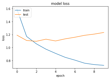
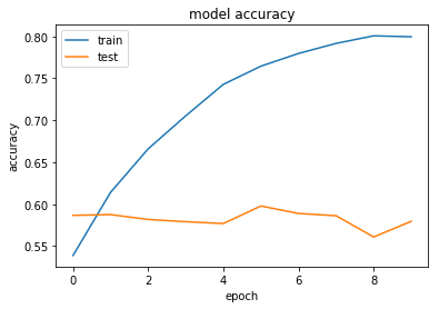
This seems to work a little bit better - but there is about 2-3% variance so it is difficult to tell. Maybe we can try to train for a number of additional epochs.

from keras.layers import Dropout

def keras_dropout_model():
    # create model
    model = Sequential()
    model.add(Dropout(0.5, input_shape=(input_dim,)))
    model.add(Dense(500, activation='relu'))
    model.add(Dropout(0.5))
    model.add(Dense(no_classes, activation='softmax'))
    # Compile model
    model.compile(loss='categorical_crossentropy', optimizer='adam', metrics=['accuracy'])
    return model

model = keras_dropout_model()
model.summary()
history = model.fit(X, Y, validation_split=0.2, epochs=20, batch_size=5, verbose=1)

# list all data in history
print(history.history.keys())
# summarize history for accuracy
plt.plot(history.history['acc'])
plt.plot(history.history['val_acc'])
plt.title('model accuracy')
plt.ylabel('accuracy')
plt.xlabel('epoch')
plt.legend(['train', 'test'], loc='upper left')
plt.show()
# summarize history for loss
plt.plot(history.history['loss'])
plt.plot(history.history['val_loss'])
plt.title('model loss')
plt.ylabel('loss')
plt.xlabel('epoch')
plt.legend(['train', 'test'], loc='upper left')
plt.show()

_________________________________________________________________
Layer (type)                 Output Shape              Param #   
=================================================================
dropout_5 (Dropout)          (None, 5000)              0         
_________________________________________________________________
dense_15 (Dense)             (None, 500)               2500500   
_________________________________________________________________
dropout_6 (Dropout)          (None, 500)               0         
_________________________________________________________________
dense_16 (Dense)             (None, 8)                 4008      
=================================================================
Total params: 2,504,508
Trainable params: 2,504,508
Non-trainable params: 0
_________________________________________________________________
Train on 8990 samples, validate on 2248 samples
Epoch 1/20
8990/8990 [==============================] - 278s - loss: 1.6090 - acc: 0.4763 - val_loss: 1.1685 - val_acc: 0.6005
Epoch 2/20
8990/8990 [==============================] - 283s - loss: 1.1541 - acc: 0.6034 - val_loss: 1.1139 - val_acc: 0.6241
Epoch 3/20
8990/8990 [==============================] - 285s - loss: 1.0295 - acc: 0.6519 - val_loss: 1.1211 - val_acc: 0.6192
Epoch 4/20
8990/8990 [==============================] - 260s - loss: 0.9636 - acc: 0.6799 - val_loss: 1.1416 - val_acc: 0.6219
Epoch 5/20
8990/8990 [==============================] - 259s - loss: 0.9235 - acc: 0.6949 - val_loss: 1.1070 - val_acc: 0.6157
Epoch 6/20
8990/8990 [==============================] - 259s - loss: 0.8431 - acc: 0.7226 - val_loss: 1.1461 - val_acc: 0.6125
Epoch 7/20
8990/8990 [==============================] - 259s - loss: 0.7866 - acc: 0.7433 - val_loss: 1.1609 - val_acc: 0.6237
Epoch 8/20
8990/8990 [==============================] - 258s - loss: 0.7834 - acc: 0.7493 - val_loss: 1.1745 - val_acc: 0.6272
Epoch 9/20
8990/8990 [==============================] - 258s - loss: 0.7383 - acc: 0.7671 - val_loss: 1.1679 - val_acc: 0.6232
Epoch 10/20
8990/8990 [==============================] - 324s - loss: 0.7204 - acc: 0.7705 - val_loss: 1.2209 - val_acc: 0.6192
Epoch 11/20
8990/8990 [==============================] - 321s - loss: 0.7308 - acc: 0.7707 - val_loss: 1.2136 - val_acc: 0.6188
Epoch 12/20
8990/8990 [==============================] - 312s - loss: 0.6907 - acc: 0.7908 - val_loss: 1.2437 - val_acc: 0.6241
Epoch 13/20
8990/8990 [==============================] - 325s - loss: 0.6700 - acc: 0.7973 - val_loss: 1.2450 - val_acc: 0.6272
Epoch 14/20
8990/8990 [==============================] - 298s - loss: 0.6431 - acc: 0.8097 - val_loss: 1.2810 - val_acc: 0.6197
Epoch 15/20
8990/8990 [==============================] - 324s - loss: 0.6202 - acc: 0.8110 - val_loss: 1.3603 - val_acc: 0.6036
Epoch 16/20
8990/8990 [==============================] - 296s - loss: 0.6130 - acc: 0.8127 - val_loss: 1.3270 - val_acc: 0.6174
Epoch 17/20
8990/8990 [==============================] - 326s - loss: 0.6338 - acc: 0.8135 - val_loss: 1.3408 - val_acc: 0.6121
Epoch 18/20
8990/8990 [==============================] - 314s - loss: 0.6336 - acc: 0.8219 - val_loss: 1.3723 - val_acc: 0.6192
Epoch 19/20
8990/8990 [==============================] - 314s - loss: 0.5931 - acc: 0.8304 - val_loss: 1.3888 - val_acc: 0.6094
Epoch 20/20
8990/8990 [==============================] - 343s - loss: 0.6129 - acc: 0.8259 - val_loss: 1.3998 - val_acc: 0.6148
dict_keys(['val_acc', 'acc', 'loss', 'val_loss'])

png

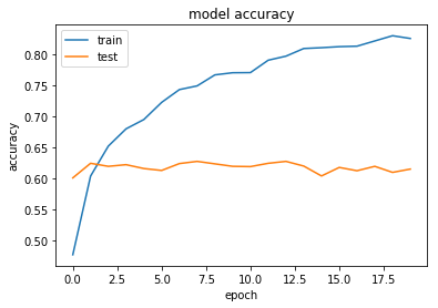
Okay so Dropout doesn't appear to improve our performance. Overfitting still occurs over time and the test accuracy appears stubbornly fixed at around 60-62%.

Improving Performance with Algorithm Tuning

Let's explore a few architecture choices with our keras model to see if we can see any improvement. At this stage we are just looking for low-hanging fruit. If a particular direction looks promising, there is the option to use grid search routines to find optimal parameters.

def keras_multi_layer_model():
    # create model
    model = Sequential()
    model.add(Dense(1000, input_dim=input_dim, activation='relu'))
    model.add(Dense(500, activation='relu'))
    model.add(Dense(250, activation='relu'))
    model.add(Dense(no_classes, activation='softmax'))
    # Compile model
    model.compile(loss='categorical_crossentropy', optimizer='adam', metrics=['accuracy'])
    return model

model = keras_multi_layer_model()
model.summary()
history = model.fit(X, Y, validation_split=0.2, epochs=10, batch_size=5, verbose=1)

# list all data in history
print(history.history.keys())
# summarize history for accuracy
plt.plot(history.history['acc'])
plt.plot(history.history['val_acc'])
plt.title('model accuracy')
plt.ylabel('accuracy')
plt.xlabel('epoch')
plt.legend(['train', 'test'], loc='upper left')
plt.show()
# summarize history for loss
plt.plot(history.history['loss'])
plt.plot(history.history['val_loss'])
plt.title('model loss')
plt.ylabel('loss')
plt.xlabel('epoch')
plt.legend(['train', 'test'], loc='upper left')
plt.show()

_________________________________________________________________
Layer (type)                 Output Shape              Param #   
=================================================================
dense_17 (Dense)             (None, 1000)              5001000   
_________________________________________________________________
dense_18 (Dense)             (None, 500)               500500    
_________________________________________________________________
dense_19 (Dense)             (None, 250)               125250    
_________________________________________________________________
dense_20 (Dense)             (None, 8)                 2008      
=================================================================
Total params: 5,628,758
Trainable params: 5,628,758
Non-trainable params: 0
_________________________________________________________________
Train on 8990 samples, validate on 2248 samples
Epoch 1/10
8990/8990 [==============================] - 647s - loss: 1.2164 - acc: 0.5645 - val_loss: 1.0894 - val_acc: 0.6277
Epoch 2/10
8990/8990 [==============================] - 632s - loss: 0.5716 - acc: 0.7991 - val_loss: 1.2262 - val_acc: 0.5952
Epoch 3/10
8990/8990 [==============================] - 631s - loss: 0.2023 - acc: 0.9385 - val_loss: 1.9201 - val_acc: 0.6085
Epoch 4/10
8990/8990 [==============================] - 664s - loss: 0.0728 - acc: 0.9806 - val_loss: 2.3951 - val_acc: 0.6214
Epoch 5/10
8990/8990 [==============================] - 634s - loss: 0.0720 - acc: 0.9858 - val_loss: 2.7070 - val_acc: 0.6183
Epoch 6/10
8990/8990 [==============================] - 636s - loss: 0.0561 - acc: 0.9892 - val_loss: 3.1284 - val_acc: 0.6059
Epoch 7/10
8990/8990 [==============================] - 635s - loss: 0.0662 - acc: 0.9899 - val_loss: 3.1941 - val_acc: 0.5988
Epoch 8/10
8990/8990 [==============================] - 643s - loss: 0.0495 - acc: 0.9918 - val_loss: 3.4484 - val_acc: 0.6130
Epoch 9/10
8990/8990 [==============================] - 635s - loss: 0.0384 - acc: 0.9938 - val_loss: 3.5622 - val_acc: 0.6134
Epoch 10/10
8990/8990 [==============================] - 635s - loss: 0.0292 - acc: 0.9961 - val_loss: 3.8888 - val_acc: 0.6117
dict_keys(['val_acc', 'acc', 'loss', 'val_loss'])

png

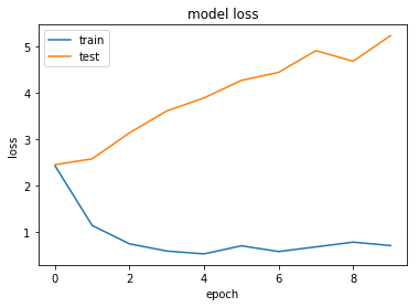
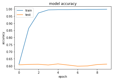
Regularisation

One method of attempting to avoid overfitting is to limit the magnitude of our weights using regularisation. This is explained in this post.

Here we will try L2 regularisation, which penalises large weight values.

from keras.regularizers import l2 # L2-regularisation
l2_lambda = 0.01

def keras_reg_model():
    # create model
    model = Sequential()
    model.add(Dense(500, input_dim=input_dim, activation='relu', kernel_regularizer=l2(l2_lambda)))
    model.add(Dense(no_classes, activation='softmax'))
    # Compile model
    model.compile(loss='categorical_crossentropy', optimizer='adam', metrics=['accuracy'])
    return model

model = keras_reg_model()
model.summary()
history = model.fit(X, Y, validation_split=0.2, epochs=10, batch_size=5, verbose=1)

# list all data in history
print(history.history.keys())
# summarize history for accuracy
plt.plot(history.history['acc'])
plt.plot(history.history['val_acc'])
plt.title('model accuracy')
plt.ylabel('accuracy')
plt.xlabel('epoch')
plt.legend(['train', 'test'], loc='upper left')
plt.show()
# summarize history for loss
plt.plot(history.history['loss'])
plt.plot(history.history['val_loss'])
plt.title('model loss')
plt.ylabel('loss')
plt.xlabel('epoch')
plt.legend(['train', 'test'], loc='upper left')
plt.show()

_________________________________________________________________
Layer (type)                 Output Shape              Param #   
=================================================================
dense_23 (Dense)             (None, 500)               2500500   
_________________________________________________________________
dense_24 (Dense)             (None, 8)                 4008      
=================================================================
Total params: 2,504,508
Trainable params: 2,504,508
Non-trainable params: 0
_________________________________________________________________
Train on 8990 samples, validate on 2248 samples
Epoch 1/10
8990/8990 [==============================] - 578s - loss: 3.8866 - acc: 0.5388 - val_loss: 2.7980 - val_acc: 0.5867
Epoch 2/10
8990/8990 [==============================] - 723s - loss: 2.6364 - acc: 0.6141 - val_loss: 2.6501 - val_acc: 0.5876
Epoch 3/10
8990/8990 [==============================] - 667s - loss: 2.1624 - acc: 0.6660 - val_loss: 2.5055 - val_acc: 0.5819
Epoch 4/10
8990/8990 [==============================] - 594s - loss: 1.7579 - acc: 0.7053 - val_loss: 2.2376 - val_acc: 0.5792
Epoch 5/10
8990/8990 [==============================] - 587s - loss: 1.5254 - acc: 0.7428 - val_loss: 2.1618 - val_acc: 0.5770
Epoch 6/10
8990/8990 [==============================] - 598s - loss: 1.3854 - acc: 0.7645 - val_loss: 2.0072 - val_acc: 0.5979
Epoch 7/10
8990/8990 [==============================] - 559s - loss: 1.2818 - acc: 0.7796 - val_loss: 2.0247 - val_acc: 0.5890
Epoch 8/10
8990/8990 [==============================] - 530s - loss: 1.2330 - acc: 0.7917 - val_loss: 2.0380 - val_acc: 0.5863
Epoch 9/10
8990/8990 [==============================] - 530s - loss: 1.1755 - acc: 0.8007 - val_loss: 2.0731 - val_acc: 0.5609
Epoch 10/10
8990/8990 [==============================] - 571s - loss: 1.1802 - acc: 0.7996 - val_loss: 2.0386 - val_acc: 0.5796
dict_keys(['val_acc', 'acc', 'loss', 'val_loss'])

png

Regularisation appears to work here. While it doesn't affect accuracy, we do now have the loss for both the train and test sets decreasing over time.

Increasing Performance with Data

Here are some steps we can try to improve performance by modifying our initial data: 1. Normalise the data - it may be worth looking into whether we can normalise our input X matrix values data to scale between 0 and 1. Our Y vector is already in a one-hot format and so cannot be normalised. 2. Changing our X dimensionality - is there any benefit in increasing or decreasing the dimensionality of our input data. For example, we can change the vocubulary cap on our text tokeniser. 3. Get more data - we have more data available and so we can maybe up our dataset to 50,000 randomly selected claims, or use each claim in each claimset as a data sample. The reason why we have tried to limit our dataset is due to time and memory concerns - if we up our dataset size these may need to be looked at. 4. Changing the form of our input data - what happens if we use (normalised) term frequency instead of TD-IDF? Could we represent our text data as a continuous bag of words (e.g. a sum of word vectors)?

Normalising the Data

We can first try to zero-center the data by substracting the mean and dividing by the standard deviation.

Now, we should note that our data is already normalised to a certain extent by the inverse document frequency term. But it may be that zero-centered data provides improvement.

X[0][0:10]

array([ 0.        ,  0.        ,  2.43021996,  2.08331543,  1.71570602,
        2.52741068,  4.87087867,  2.99092954,  2.24937914,  0.        ])

X_zero = X
X_zero -= np.mean(X_zero, axis = 0)
X_zero /= np.std(X, axis = 0)
X_zero[0][0:10]

/usr/local/lib/python3.5/dist-packages/ipykernel_launcher.py:3: RuntimeWarning: invalid value encountered in true_divide
  This is separate from the ipykernel package so we can avoid doing imports until





array([        nan, -2.22009656,  0.82212546,  0.62343302,  0.41434569,
        1.39141984,  2.02709972,  2.37849159,  1.34165113, -0.63808578])

X_zero = np.nan_to_num(X_zero, copy=False)
X_zero[0][0:10]

array([ 0.        , -2.22009656,  0.82212546,  0.62343302,  0.41434569,
        1.39141984,  2.02709972,  2.37849159,  1.34165113, -0.63808578])

model2 = keras_model()
model2.summary()
history = model2.fit(X_zero, Y, validation_split=0.2, epochs=10, batch_size=5, verbose=1)

# list all data in history
print(history.history.keys())
# summarize history for accuracy
plt.plot(history.history['acc'])
plt.plot(history.history['val_acc'])
plt.title('model accuracy')
plt.ylabel('accuracy')
plt.xlabel('epoch')
plt.legend(['train', 'test'], loc='upper left')
plt.show()
# summarize history for loss
plt.plot(history.history['loss'])
plt.plot(history.history['val_loss'])
plt.title('model loss')
plt.ylabel('loss')
plt.xlabel('epoch')
plt.legend(['train', 'test'], loc='upper left')
plt.show()

_________________________________________________________________
Layer (type)                 Output Shape              Param #   
=================================================================
dense_21 (Dense)             (None, 500)               2500500   
_________________________________________________________________
dense_22 (Dense)             (None, 8)                 4008      
=================================================================
Total params: 2,504,508
Trainable params: 2,504,508
Non-trainable params: 0
_________________________________________________________________
Train on 8990 samples, validate on 2248 samples
Epoch 1/10
8990/8990 [==============================] - 333s - loss: 2.4311 - acc: 0.5186 - val_loss: 2.4488 - val_acc: 0.5498
Epoch 2/10
8990/8990 [==============================] - 324s - loss: 1.1410 - acc: 0.7861 - val_loss: 2.5771 - val_acc: 0.5885
Epoch 3/10
8990/8990 [==============================] - 306s - loss: 0.7450 - acc: 0.8897 - val_loss: 3.1360 - val_acc: 0.5863
Epoch 4/10
8990/8990 [==============================] - 306s - loss: 0.5897 - acc: 0.9353 - val_loss: 3.6081 - val_acc: 0.5792
Epoch 5/10
8990/8990 [==============================] - 323s - loss: 0.5283 - acc: 0.9505 - val_loss: 3.8894 - val_acc: 0.5721
Epoch 6/10
8990/8990 [==============================] - 311s - loss: 0.7029 - acc: 0.9344 - val_loss: 4.2661 - val_acc: 0.5752
Epoch 7/10
8990/8990 [==============================] - 295s - loss: 0.5793 - acc: 0.9489 - val_loss: 4.4400 - val_acc: 0.5725
Epoch 8/10
8990/8990 [==============================] - 302s - loss: 0.6794 - acc: 0.9425 - val_loss: 4.9078 - val_acc: 0.5707
Epoch 9/10
8990/8990 [==============================] - 314s - loss: 0.7816 - acc: 0.9354 - val_loss: 4.6792 - val_acc: 0.5827
Epoch 10/10
8990/8990 [==============================] - 328s - loss: 0.7082 - acc: 0.9455 - val_loss: 5.2317 - val_acc: 0.5534
dict_keys(['val_acc', 'acc', 'loss', 'val_loss'])

png

Normalising our data does not seem to have any significant effect. This is to be expected - our data is already normalised to a certain extent, and we are dealing with sparse language data rather than continuous image data.

This processing does appear to help slightly to reduce overfitting. This maybe suggests that regularisation may be useful.

Changing Input Dimensionality

Let's see if increasing or decreasing the dimensionality of our input data affects our classification results. We can do this by changing the number of words cap that is passed to our tokeniser.

import pickle
with open("raw_data.pkl", "rb") as f:
    print("Loading data")
    raw_data = pickle.load(f)
    print("{0} claims and classifications loaded".format(len(data)))

Loading data
11238 claims and classifications loaded

# Create our Y vector as before
from keras.utils import to_categorical
from sklearn.preprocessing import LabelEncoder

Y_class = [d[1] for d in raw_data]

# encode class values as integers
label_e = LabelEncoder()
label_e.fit(Y_class)
encoded_Y = label_e.transform(Y_class)
# convert integers to dummy variables (i.e. one hot encoded)
Y = to_categorical(encoded_Y)
print("Our classes are now a matrix of {0}".format(Y.shape))
print("Original label: {0}; Converted label: {1}".format(Y_class[0], Y[0]))

Our classes are now a matrix of (11238, 8)
Original label: A; Converted label: [1. 0. 0. 0. 0. 0. 0. 0.]

# Let's start with decreasing our dimensionality

from keras.preprocessing.text import Tokenizer

docs = [d[0] for d in raw_data]

# create the tokenizer
t = Tokenizer(num_words=2500)
# fit the tokenizer on the documents
t.fit_on_texts(docs)

X = t.texts_to_matrix(docs, mode='tfidf')
print("Our data has the following dimensionality: ", X.shape)

Our data has the following dimensionality:  (11238, 2500)

We are going to leave our SVC classifier for these experiments as it took too long to train.

import numpy
from sklearn.model_selection import cross_val_score
from sklearn.naive_bayes import MultinomialNB
from sklearn.neural_network import MLPClassifier

classifiers = [
    MultinomialNB(),
    MLPClassifier()
]

results = list()
# Convert one hot to target integer
Y_integers = numpy.argmax(Y, axis=1)

for clf in classifiers:
    name = clf.__class__.__name__
    scores = cross_val_score(clf, X, Y_integers, cv=5)
    results.append((
        name, 
        scores.mean()*100, 
        scores.std()*100
    ))

    print(
        "Classifier {0} has an average classification accuracy of {1:.2f} ({2:.2f})".format(
            name, 
            scores.mean()*100, 
            scores.std()*100
        )    
    )

Classifier MultinomialNB has an average classification accuracy of 57.04 (0.97)
Classifier MLPClassifier has an average classification accuracy of 60.17 (1.07)

Here are our results:

Classifier MultinomialNB has an average classification accuracy of 57.04 (0.97)
Classifier MLPClassifier has an average classification accuracy of 60.17 (1.07)

Comparing with our previous results:

Classifier MultinomialNB has an average classification accuracy of 58.90 (1.12)
Classifier MLPClassifier has an average classification accuracy of 61.20 (0.54)

We see a slight reduction in accuracy, although we are on or close to the bounds of variance. Reducing our dimensionality does not seem to be the way to proceed.

Even though our SVC classifier performed well in the spot-checks - it takes a very long time to train. For these more general experiments, we will thus limit to the Naive Bayes and the MLP classifier.

# Now let's increase our dimensionality

# Delete our earlier data
del X, t

from keras.preprocessing.text import Tokenizer

# create the tokenizer
t = Tokenizer(num_words=10000)
# fit the tokenizer on the documents
t.fit_on_texts(docs)

X = t.texts_to_matrix(docs, mode='tfidf')
print("Our data has the following dimensionality: ", X.shape)

# SVC takes too long to train
classifiers = [
    MultinomialNB(),
    MLPClassifier()
]
for clf in classifiers:
    name = clf.__class__.__name__
    scores = cross_val_score(clf, X, Y_integers, cv=5)
    results.append((
        name, 
        scores.mean()*100, 
        scores.std()*100
    ))

    print(
        "Classifier {0} has an average classification accuracy of {1:.2f} ({2:.2f})".format(
            name, 
            scores.mean()*100, 
            scores.std()*100
        )    
    )

Our data has the following dimensionality:  (11238, 10000)
Classifier MultinomialNB has an average classification accuracy of 59.26 (1.16)
Classifier MLPClassifier has an average classification accuracy of 62.11 (0.36)

Results:

Classifier MultinomialNB has an average classification accuracy of 59.26 (1.16)
Classifier MLPClassifier has an average classification accuracy of 62.11 (0.36)

There does appear to be a small increase in performance (~2% - where variance is ~1%). So more words does help us. However, it does not help as much as we would expect it too (e.g. doubling our number of counted words does not double performance).

This indicates that much of our classification is being performed on a limited set of terms.

Let's see what another doubling of our dimensionality does...

# Delete our earlier data
del X, t

from keras.preprocessing.text import Tokenizer

# create the tokenizer
t = Tokenizer(num_words=20000)
# fit the tokenizer on the documents
t.fit_on_texts(docs)

X = t.texts_to_matrix(docs, mode='tfidf')
print("Our data has the following dimensionality: ", X.shape)

# SVC takes too long to train
classifiers = [
    MultinomialNB(),
    MLPClassifier()
]
for clf in classifiers:
    name = clf.__class__.__name__
    scores = cross_val_score(clf, X, Y_integers, cv=5)
    results.append((
        name, 
        scores.mean()*100, 
        scores.std()*100
    ))

    print(
        "Classifier {0} has an average classification accuracy of {1:.2f} ({2:.2f})".format(
            name, 
            scores.mean()*100, 
            scores.std()*100
        )    
    )

Our data has the following dimensionality:  (11238, 20000)
Classifier MultinomialNB has an average classification accuracy of 59.24 (1.33)
Classifier MLPClassifier has an average classification accuracy of 61.91 (0.43)

Results:

Classifier MultinomialNB has an average classification accuracy of 59.24 (1.33)
Classifier MLPClassifier has an average classification accuracy of 61.91 (0.43)

There seems to be a leveling off of performance with increased dimensionality. Here there will always be a trade-off between dimensionality and performance. In this case, as we are only obtaining a small percentage increase, it may be better to use a smaller dimensionality to allow faster classification.

Another aside on speed: the Naive Bayes classifier is much faster to train than the MLP classifier, and the difference in performance is only 1-2%. If we were looking at a production system, there may be a benefit in using the Naive Bayes classifier over the more fancy deep-learning approaches.

Changing Data Conversion Methods

The texts_to_matrix method for the text tokeniser has for different modes: "binary", "count", "tfidf", "freq". These are not explained but it is presumed that binary provides just an indication of presence for a word, and count/freq provide un-normalised count data. Looking at the source, freq divides the count c by the length of the sequence.

modes = ["binary", "count", "freq"]

for mode in modes:
    # create the tokenizer
    t = Tokenizer(num_words=5000)
    # fit the tokenizer on the documents
    t.fit_on_texts(docs)

    X = t.texts_to_matrix(docs, mode=mode)
    for clf in classifiers:
        name = clf.__class__.__name__
        scores = cross_val_score(clf, X, Y_integers, cv=5)

        print(
            "Mode {0} - Classifier {1} has an average classification accuracy of {2:.2f} ({3:.2f})".format(
                mode,
                name, 
                scores.mean()*100, 
                scores.std()*100
            )    
        )

Mode binary - Classifier MultinomialNB has an average classification accuracy of 57.07 (0.82)
Mode binary - Classifier MLPClassifier has an average classification accuracy of 59.63 (0.71)
Mode count - Classifier MultinomialNB has an average classification accuracy of 57.53 (0.89)
Mode count - Classifier MLPClassifier has an average classification accuracy of 59.00 (0.63)
Mode freq - Classifier MultinomialNB has an average classification accuracy of 30.82 (0.05)
Mode freq - Classifier MLPClassifier has an average classification accuracy of 57.65 (1.38)

Results:

Mode binary - Classifier MultinomialNB has an average classification accuracy of 57.07 (0.82)
Mode binary - Classifier MLPClassifier has an average classification accuracy of 59.63 (0.71)
Mode count - Classifier MultinomialNB has an average classification accuracy of 57.53 (0.89)
Mode count - Classifier MLPClassifier has an average classification accuracy of 59.00 (0.63)
Mode freq - Classifier MultinomialNB has an average classification accuracy of 30.82 (0.05)
Mode freq - Classifier MLPClassifier has an average classification accuracy of 57.65 (1.38)

Some interestings results here. TD-IDF appears the best metric to use. Frequency counts appear to cause problems with both classifiers (the MLP does not converge to a solution after 200 iterations). Using TD-IDF over just count data appears to increase performance by 1-2%.

Getting More Data

Let's see what happens when we try 20,000 claims.

At the moment the interface for getting the data is a little slow...

# Now try 20,000 patent publications at random

import os, pickle

from collections import Counter

# Get the claim 1 and classificationt text

PIK = "claim_and_class20k.data"

if os.path.isfile(PIK):
    with open(PIK, "rb") as f:
        print("Loading data")
        data = pickle.load(f)
        print("{0} claims and classifications loaded".format(len(data)))
else:
    from patentdata.corpus import USPublications
    from patentdata.models.patentcorpus import LazyPatentCorpus

    path = '/patentdata/media/SAMSUNG1/Patent_Downloads'
    ds = USPublications(path)

    lzy = LazyPatentCorpus(ds, sample_size=20000)

    data = list()
    for i, pd in enumerate(lzy):
        try:
            classifications = [c.as_string() for c in pd.classifications]
        except:
            classifications = ""
        try:
            claim1_text = pd.claimset.get_claim(1).text
        except:
            claim1_text = ""
        current_data = (claim1_text, classifications)
        data.append(current_data)
        if (i % 500) == 0:
            print("Saving a checkpoint at {0} files".format(i))
            print("Current data = ", pd.title)
            with open(PIK, "wb") as f:
                pickle.dump(data, f)

    with open(PIK, "wb") as f:
        pickle.dump(data, f)

    print("{0} claims saved".format(len(data)))

Loading data
19001 claims and classifications loaded

We got a memory error after 19000 but that is still more data than we had before. Let's use that. You can find the "claim_and_class20k.data" file in the GitHub directory if you want to load the data yourself.

PIK = "raw_data20k.pkl"

if os.path.isfile(PIK):
    with open(PIK, "rb") as f:
        print("Loading data")
        data = pickle.load(f)
else:
    # Check for and remove 'cancelled' claims
    data = [d for d in data if '(canceled)' not in d[0]]
    cleaner_data = list()
    for d in data:
        if len(d[1]) >= 1:
            if len(d[1][0]) > 3:
                classification = d[1][0][2]
                cleaner_data.append(
                    (d[0], classification)
                )
    data = cleaner_data

    from patentdata.models.lib.utils import clean_characters

    data = [(clean_characters(d[0]), d[1]) for d in data]

    with open("raw_data20k.pkl", "wb") as f:
        pickle.dump(data, f)

Loading data

print("We have {0} data samples left after cleaning.".format(len(data)))

We have 17712 data samples left after cleaning.

from keras.utils import to_categorical
from sklearn.preprocessing import LabelEncoder

Y_class = [d[1] for d in data]

# encode class values as integers
label_e = LabelEncoder()
label_e.fit(Y_class)
encoded_Y = label_e.transform(Y_class)
# convert integers to dummy variables (i.e. one hot encoded)
Y = to_categorical(encoded_Y)
print("Our classes are now a matrix of {0}".format(Y.shape))
print("Original label: {0}; Converted label: {1}".format(Y_class[0], Y[0]))

from keras.preprocessing.text import Tokenizer

docs = [d[0] for d in data]

# create the tokenizer
t = Tokenizer(num_words=5000)
# fit the tokenizer on the documents
t.fit_on_texts(docs)

X = t.texts_to_matrix(docs, mode='tfidf')

print("Our data has the following dimensionality: ", X.shape)
print("An example array is: ", X[0][0:100])

Our classes are now a matrix of (17712, 8)
Original label: G; Converted label: [0. 0. 0. 0. 0. 0. 1. 0.]
Our data has the following dimensionality:  (17712, 5000)
An example array is:  [0.         2.19509726 1.66470012 0.         1.21538639 1.66504906
 0.         0.88406116 0.         0.         1.66670622 0.69334485
 0.         0.75089151 0.         0.         1.47841041 1.27422143
 1.15174037 0.         0.         0.         0.         0.
 2.9039738  0.         0.         0.         0.         0.
 0.         0.         0.         0.         0.         0.
 0.         1.93181596 0.         0.         0.         0.
 0.         0.         0.         0.         0.         2.27206512
 0.         1.95791029 0.         0.         2.3501247  0.
 0.         0.         0.         0.         0.         0.
 0.         0.         0.         0.         0.         0.
 0.         0.         5.8289026  0.         0.         0.
 0.         0.         0.         0.         0.         0.
 0.         0.         0.         0.         0.         0.
 4.79273481 0.         0.         0.         0.         0.
 0.         0.         0.         3.04409238 0.         0.
 0.         0.         2.44064762 0.        ]

with open("encoded_data20k.pkl", "wb") as f:
    pickle.dump((X, Y), f)

import numpy
from sklearn.model_selection import cross_val_score
from sklearn.naive_bayes import MultinomialNB
from sklearn.neural_network import MLPClassifier

classifiers = [
    MultinomialNB(),
    MLPClassifier()
]

results = list()
# Convert one hot to target integer
Y_integers = numpy.argmax(Y, axis=1)

for clf in classifiers:
    name = clf.__class__.__name__
    scores = cross_val_score(clf, X, Y_integers, cv=5)
    results.append((
        name, 
        scores.mean()*100, 
        scores.std()*100
    ))

    print(
        "Classifier {0} has an average classification accuracy of {1:.2f} ({2:.2f})".format(
            name, 
            scores.mean()*100, 
            scores.std()*100
        )    
    )

Results:

Classifier MultinomialNB has an average classification accuracy of 58.22 (0.34)
Classifier MLPClassifier has an average classification accuracy of 62.38 (0.88)

So possibly a very small improvement but well within the realms of statistical variance. Let us see if more data helps with our keras model.

from keras.models import Sequential
from keras.layers import Dense, Activation, Dropout
import matplotlib.pyplot as plt

input_dim = X.shape[1]
print("Our input dimension for our claim representation is {0}".format(input_dim))

no_classes = Y.shape[1]
print("Our output dimension is {0}".format(no_classes))

Our input dimension for our claim representation is 5000
Our output dimension is 8

def keras_model():
    # create model
    model = Sequential()
    model.add(Dense(500, input_dim=input_dim, activation='relu'))
    model.add(Dense(no_classes, activation='softmax'))
    # Compile model
    model.compile(loss='categorical_crossentropy', optimizer='adam', metrics=['accuracy'])
    return model


model = keras_model()
model.summary()
history = model.fit(X, Y, validation_split=0.2, epochs=10, batch_size=5, verbose=1)

# list all data in history
print(history.history.keys())
# summarize history for accuracy
plt.plot(history.history['acc'])
plt.plot(history.history['val_acc'])
plt.title('model accuracy')
plt.ylabel('accuracy')
plt.xlabel('epoch')
plt.legend(['train', 'test'], loc='upper left')
plt.show()
# summarize history for loss
plt.plot(history.history['loss'])
plt.plot(history.history['val_loss'])
plt.title('model loss')
plt.ylabel('loss')
plt.xlabel('epoch')
plt.legend(['train', 'test'], loc='upper left')
plt.show()

Our input dimension for our claim representation is 5000
Our output dimension is 8
_________________________________________________________________
Layer (type)                 Output Shape              Param #   
=================================================================
dense_1 (Dense)              (None, 500)               2500500   
_________________________________________________________________
dense_2 (Dense)              (None, 8)                 4008      
=================================================================
Total params: 2,504,508
Trainable params: 2,504,508
Non-trainable params: 0
_________________________________________________________________
Train on 14169 samples, validate on 3543 samples
Epoch 1/10
14169/14169 [==============================] - 530s - loss: 1.1325 - acc: 0.6120 - val_loss: 1.0894 - val_acc: 0.6077
Epoch 2/10
14169/14169 [==============================] - 475s - loss: 0.3948 - acc: 0.8646 - val_loss: 1.4186 - val_acc: 0.6105
Epoch 3/10
14169/14169 [==============================] - 566s - loss: 0.1108 - acc: 0.9724 - val_loss: 1.9858 - val_acc: 0.6113
Epoch 4/10
14169/14169 [==============================] - 454s - loss: 0.0334 - acc: 0.9939 - val_loss: 2.3294 - val_acc: 0.6065
Epoch 5/10
14169/14169 [==============================] - 476s - loss: 0.0283 - acc: 0.9960 - val_loss: 2.5955 - val_acc: 0.6139
Epoch 6/10
14169/14169 [==============================] - 513s - loss: 0.0250 - acc: 0.9960 - val_loss: 2.8697 - val_acc: 0.6063
Epoch 7/10
14169/14169 [==============================] - 457s - loss: 0.0223 - acc: 0.9968 - val_loss: 3.2368 - val_acc: 0.5981
Epoch 8/10
14169/14169 [==============================] - 449s - loss: 0.0178 - acc: 0.9977 - val_loss: 3.3843 - val_acc: 0.5995
Epoch 9/10
14169/14169 [==============================] - 430s - loss: 0.0177 - acc: 0.9976 - val_loss: 3.4755 - val_acc: 0.6094
Epoch 10/10
14169/14169 [==============================] - 427s - loss: 0.0141 - acc: 0.9984 - val_loss: 3.5041 - val_acc: 0.6125
dict_keys(['val_loss', 'val_acc', 'loss', 'acc'])

png

Our accuracy appears to have improved by 1-2%. This is still a small increase though, and possibly within the variance of our classifier. Let's try with regularisation, which had the best effect to prevent overfitting.

from keras.regularizers import l2 # L2-regularisation
l2_lambda = 0.1

def keras_reg_model():
    # create model
    model = Sequential()
    model.add(Dense(500, input_dim=input_dim, activation='relu', kernel_regularizer=l2(l2_lambda)))
    model.add(Dense(no_classes, activation='softmax'))
    # Compile model
    model.compile(loss='categorical_crossentropy', optimizer='adam', metrics=['accuracy'])
    return model

model = keras_reg_model()
model.summary()
history = model.fit(X, Y, validation_split=0.2, epochs=10, batch_size=5, verbose=1)

# list all data in history
print(history.history.keys())
# summarize history for accuracy
plt.plot(history.history['acc'])
plt.plot(history.history['val_acc'])
plt.title('model accuracy')
plt.ylabel('accuracy')
plt.xlabel('epoch')
plt.legend(['train', 'test'], loc='upper left')
plt.show()
# summarize history for loss
plt.plot(history.history['loss'])
plt.plot(history.history['val_loss'])
plt.title('model loss')
plt.ylabel('loss')
plt.xlabel('epoch')
plt.legend(['train', 'test'], loc='upper left')
plt.show()

_________________________________________________________________
Layer (type)                 Output Shape              Param #   
=================================================================
dense_3 (Dense)              (None, 500)               2500500   
_________________________________________________________________
dense_4 (Dense)              (None, 8)                 4008      
=================================================================
Total params: 2,504,508
Trainable params: 2,504,508
Non-trainable params: 0
_________________________________________________________________
Train on 14169 samples, validate on 3543 samples
Epoch 1/10
14169/14169 [==============================] - 1109s - loss: 3.5127 - acc: 0.5249 - val_loss: 2.8284 - val_acc: 0.5174
Epoch 2/10
14169/14169 [==============================] - 911s - loss: 2.5778 - acc: 0.5597 - val_loss: 2.4618 - val_acc: 0.5577
Epoch 3/10
14169/14169 [==============================] - 905s - loss: 2.2790 - acc: 0.5762 - val_loss: 2.1673 - val_acc: 0.5555
Epoch 4/10
14169/14169 [==============================] - 930s - loss: 2.1328 - acc: 0.5876 - val_loss: 2.1349 - val_acc: 0.5642
Epoch 5/10
14169/14169 [==============================] - 943s - loss: 2.0365 - acc: 0.5944 - val_loss: 2.0831 - val_acc: 0.5795
Epoch 6/10
14169/14169 [==============================] - 943s - loss: 1.9580 - acc: 0.5982 - val_loss: 2.0456 - val_acc: 0.5687
Epoch 7/10
 1285/14169 [=>............................] - ETA: 866s - loss: 1.8422 - acc: 0.6661

Gvien our results so far - let's try a multilayer model with regularisation and aggressive dropout.

def keras_best_model():
    # create model
    model = Sequential()
    model.add(Dropout(0.5, input_shape=(input_dim,)))
    model.add(Dense(1000, activation='relu', kernel_regularizer=l2(l2_lambda)))
    model.add(Dropout(0.5))
    model.add(Dense(500, activation='relu', kernel_regularizer=l2(l2_lambda)))
    model.add(Dropout(0.25))
    model.add(Dense(250, activation='relu', kernel_regularizer=l2(l2_lambda)))
    model.add(Dropout(0.25))
    model.add(Dense(no_classes, activation='softmax'))
    # Compile model
    model.compile(loss='categorical_crossentropy', optimizer='adam', metrics=['accuracy'])
    return model

model = keras_best_model()
model.summary()
history = model.fit(X, Y, validation_split=0.2, epochs=10, batch_size=5, verbose=1)

# list all data in history
print(history.history.keys())
# summarize history for accuracy
plt.plot(history.history['acc'])
plt.plot(history.history['val_acc'])
plt.title('model accuracy')
plt.ylabel('accuracy')
plt.xlabel('epoch')
plt.legend(['train', 'test'], loc='upper left')
plt.show()
# summarize history for loss
plt.plot(history.history['loss'])
plt.plot(history.history['val_loss'])
plt.title('model loss')
plt.ylabel('loss')
plt.xlabel('epoch')
plt.legend(['train', 'test'], loc='upper left')
plt.show()

_________________________________________________________________
Layer (type)                 Output Shape              Param #   
=================================================================
dropout_3 (Dropout)          (None, 5000)              0         
_________________________________________________________________
dense_2 (Dense)              (None, 1000)              5001000   
_________________________________________________________________
dropout_4 (Dropout)          (None, 1000)              0         
_________________________________________________________________
dense_3 (Dense)              (None, 500)               500500    
_________________________________________________________________
dropout_5 (Dropout)          (None, 500)               0         
_________________________________________________________________
dense_4 (Dense)              (None, 250)               125250    
_________________________________________________________________
dropout_6 (Dropout)          (None, 250)               0         
_________________________________________________________________
dense_5 (Dense)              (None, 8)                 2008      
=================================================================
Total params: 5,628,758
Trainable params: 5,628,758
Non-trainable params: 0
_________________________________________________________________
Train on 14169 samples, validate on 3543 samples
Epoch 1/10
14169/14169 [==============================] - 235s 17ms/step - loss: 4.1414 - acc: 0.3485 - val_loss: 2.2931 - val_acc: 0.3796
Epoch 2/10
14169/14169 [==============================] - 235s 17ms/step - loss: 2.3008 - acc: 0.3622 - val_loss: 2.2649 - val_acc: 0.3717
Epoch 3/10
14169/14169 [==============================] - 233s 16ms/step - loss: 2.2481 - acc: 0.3641 - val_loss: 2.1900 - val_acc: 0.3853
Epoch 4/10
14169/14169 [==============================] - 234s 17ms/step - loss: 2.2471 - acc: 0.3657 - val_loss: 2.1706 - val_acc: 0.3872
Epoch 5/10
14169/14169 [==============================] - 233s 16ms/step - loss: 2.2167 - acc: 0.3652 - val_loss: 2.1241 - val_acc: 0.3915
Epoch 6/10
14169/14169 [==============================] - 228s 16ms/step - loss: 2.1903 - acc: 0.3681 - val_loss: 2.1248 - val_acc: 0.3884
Epoch 7/10
14169/14169 [==============================] - 228s 16ms/step - loss: 2.1529 - acc: 0.3649 - val_loss: 2.0640 - val_acc: 0.3810
Epoch 8/10
14169/14169 [==============================] - 233s 16ms/step - loss: 2.1292 - acc: 0.3690 - val_loss: 2.0177 - val_acc: 0.3816
Epoch 9/10
14169/14169 [==============================] - 234s 17ms/step - loss: 2.1398 - acc: 0.3700 - val_loss: 2.0846 - val_acc: 0.3929
Epoch 10/10
14169/14169 [==============================] - 237s 17ms/step - loss: 2.1281 - acc: 0.3656 - val_loss: 2.0500 - val_acc: 0.3864
dict_keys(['val_loss', 'val_acc', 'acc', 'loss'])

png

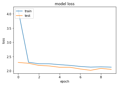
Maybe that's too aggressive on the regularisation...

l2_lambda = 0.05

def keras_best_model():
    # create model
    model = Sequential()
    model.add(Dropout(0.25, input_shape=(input_dim,)))
    model.add(Dense(1000, activation='relu', kernel_regularizer=l2(l2_lambda)))
    model.add(Dropout(0.25))
    model.add(Dense(500, activation='relu', kernel_regularizer=l2(l2_lambda)))
    model.add(Dropout(0.2))
    model.add(Dense(250, activation='relu', kernel_regularizer=l2(l2_lambda)))
    model.add(Dense(no_classes, activation='softmax'))
    # Compile model
    model.compile(loss='categorical_crossentropy', optimizer='adam', metrics=['accuracy'])
    return model

model = keras_best_model()
model.summary()
history = model.fit(X, Y, validation_split=0.2, epochs=100, batch_size=32, verbose=1)

# list all data in history
print(history.history.keys())
# summarize history for accuracy
plt.plot(history.history['acc'])
plt.plot(history.history['val_acc'])
plt.title('model accuracy')
plt.ylabel('accuracy')
plt.xlabel('epoch')
plt.legend(['train', 'test'], loc='upper left')
plt.show()
# summarize history for loss
plt.plot(history.history['loss'])
plt.plot(history.history['val_loss'])
plt.title('model loss')
plt.ylabel('loss')
plt.xlabel('epoch')
plt.legend(['train', 'test'], loc='upper left')
plt.show()

_________________________________________________________________
Layer (type)                 Output Shape              Param #   
=================================================================
dropout_2 (Dropout)          (None, 5000)              0         
_________________________________________________________________
dense_1 (Dense)              (None, 1000)              5001000   
_________________________________________________________________
dropout_3 (Dropout)          (None, 1000)              0         
_________________________________________________________________
dense_2 (Dense)              (None, 500)               500500    
_________________________________________________________________
dropout_4 (Dropout)          (None, 500)               0         
_________________________________________________________________
dense_3 (Dense)              (None, 250)               125250    
_________________________________________________________________
dense_4 (Dense)              (None, 8)                 2008      
=================================================================
Total params: 5,628,758
Trainable params: 5,628,758
Non-trainable params: 0
_________________________________________________________________
Train on 14169 samples, validate on 3543 samples
Epoch 1/100
14169/14169 [==============================] - 39s 3ms/step - loss: 7.0981 - acc: 0.4782 - val_loss: 2.0088 - val_acc: 0.4773
Epoch 2/100
14169/14169 [==============================] - 38s 3ms/step - loss: 1.9643 - acc: 0.5087 - val_loss: 2.0833 - val_acc: 0.4423
Epoch 3/100
14169/14169 [==============================] - 38s 3ms/step - loss: 1.9313 - acc: 0.5189 - val_loss: 1.8856 - val_acc: 0.5095
Epoch 4/100
14169/14169 [==============================] - 38s 3ms/step - loss: 1.8617 - acc: 0.5285 - val_loss: 1.7967 - val_acc: 0.5202
Epoch 5/100
14169/14169 [==============================] - 38s 3ms/step - loss: 1.8270 - acc: 0.5317 - val_loss: 1.8067 - val_acc: 0.5264
Epoch 6/100
14169/14169 [==============================] - 39s 3ms/step - loss: 1.8229 - acc: 0.5298 - val_loss: 1.7852 - val_acc: 0.5275
Epoch 7/100
14169/14169 [==============================] - 39s 3ms/step - loss: 1.8020 - acc: 0.5363 - val_loss: 1.7479 - val_acc: 0.5278
Epoch 8/100
14169/14169 [==============================] - 39s 3ms/step - loss: 1.7970 - acc: 0.5411 - val_loss: 1.7326 - val_acc: 0.5413
Epoch 9/100
14169/14169 [==============================] - 39s 3ms/step - loss: 1.7868 - acc: 0.5490 - val_loss: 1.7972 - val_acc: 0.5405
Epoch 10/100
14169/14169 [==============================] - 39s 3ms/step - loss: 1.8063 - acc: 0.5497 - val_loss: 1.7729 - val_acc: 0.5741
Epoch 11/100
14169/14169 [==============================] - 39s 3ms/step - loss: 1.7935 - acc: 0.5521 - val_loss: 1.7277 - val_acc: 0.5543
Epoch 12/100
14169/14169 [==============================] - 39s 3ms/step - loss: 1.7793 - acc: 0.5564 - val_loss: 1.7212 - val_acc: 0.5628
Epoch 13/100
14169/14169 [==============================] - 39s 3ms/step - loss: 1.7716 - acc: 0.5566 - val_loss: 1.7344 - val_acc: 0.5648
Epoch 14/100
14169/14169 [==============================] - 40s 3ms/step - loss: 1.7912 - acc: 0.5646 - val_loss: 1.7609 - val_acc: 0.5459
Epoch 15/100
14169/14169 [==============================] - 38s 3ms/step - loss: 1.8010 - acc: 0.5617 - val_loss: 1.7758 - val_acc: 0.5555
Epoch 16/100
14169/14169 [==============================] - 38s 3ms/step - loss: 1.7647 - acc: 0.5708 - val_loss: 1.7577 - val_acc: 0.5715
Epoch 17/100
14169/14169 [==============================] - 38s 3ms/step - loss: 1.7735 - acc: 0.5630 - val_loss: 1.7828 - val_acc: 0.5682
Epoch 18/100
14169/14169 [==============================] - 38s 3ms/step - loss: 1.7775 - acc: 0.5674 - val_loss: 1.6914 - val_acc: 0.5732
Epoch 19/100
14169/14169 [==============================] - 39s 3ms/step - loss: 1.7649 - acc: 0.5616 - val_loss: 1.7659 - val_acc: 0.5656
Epoch 20/100
14169/14169 [==============================] - 39s 3ms/step - loss: 1.7653 - acc: 0.5687 - val_loss: 1.7269 - val_acc: 0.5778
Epoch 21/100
14169/14169 [==============================] - 39s 3ms/step - loss: 1.7926 - acc: 0.5676 - val_loss: 1.7353 - val_acc: 0.5769
Epoch 22/100
14169/14169 [==============================] - 39s 3ms/step - loss: 1.8137 - acc: 0.5681 - val_loss: 1.7812 - val_acc: 0.5964
Epoch 23/100
14169/14169 [==============================] - 38s 3ms/step - loss: 1.8417 - acc: 0.5700 - val_loss: 1.8175 - val_acc: 0.5543
Epoch 24/100
14169/14169 [==============================] - 39s 3ms/step - loss: 1.7910 - acc: 0.5670 - val_loss: 1.7624 - val_acc: 0.5797
Epoch 25/100
14169/14169 [==============================] - 39s 3ms/step - loss: 1.7443 - acc: 0.5701 - val_loss: 1.7018 - val_acc: 0.5831
Epoch 26/100
14169/14169 [==============================] - 39s 3ms/step - loss: 1.7419 - acc: 0.5736 - val_loss: 1.7574 - val_acc: 0.5684
Epoch 27/100
14169/14169 [==============================] - 39s 3ms/step - loss: 1.7701 - acc: 0.5755 - val_loss: 1.7539 - val_acc: 0.5577
Epoch 28/100
14169/14169 [==============================] - 40s 3ms/step - loss: 1.7878 - acc: 0.5751 - val_loss: 1.7290 - val_acc: 0.5800
Epoch 29/100
14169/14169 [==============================] - 39s 3ms/step - loss: 1.7429 - acc: 0.5757 - val_loss: 1.7327 - val_acc: 0.5580
Epoch 30/100
14169/14169 [==============================] - 39s 3ms/step - loss: 1.7342 - acc: 0.5731 - val_loss: 1.6896 - val_acc: 0.5704
Epoch 31/100
14169/14169 [==============================] - 39s 3ms/step - loss: 1.7455 - acc: 0.5782 - val_loss: 1.6768 - val_acc: 0.5766
Epoch 32/100
14169/14169 [==============================] - 39s 3ms/step - loss: 1.7320 - acc: 0.5803 - val_loss: 1.6411 - val_acc: 0.5857
Epoch 33/100
14169/14169 [==============================] - 39s 3ms/step - loss: 1.7088 - acc: 0.5726 - val_loss: 1.6477 - val_acc: 0.5834
Epoch 34/100
14169/14169 [==============================] - 39s 3ms/step - loss: 1.7210 - acc: 0.5770 - val_loss: 1.6664 - val_acc: 0.5865
Epoch 35/100
14169/14169 [==============================] - 39s 3ms/step - loss: 1.7339 - acc: 0.5729 - val_loss: 1.7065 - val_acc: 0.5676
Epoch 36/100
14169/14169 [==============================] - 39s 3ms/step - loss: 1.7247 - acc: 0.5785 - val_loss: 1.7183 - val_acc: 0.5588
Epoch 37/100
14169/14169 [==============================] - 39s 3ms/step - loss: 1.7036 - acc: 0.5799 - val_loss: 1.6512 - val_acc: 0.5854
Epoch 38/100
14169/14169 [==============================] - 39s 3ms/step - loss: 1.6881 - acc: 0.5803 - val_loss: 1.6607 - val_acc: 0.5845
Epoch 39/100
14169/14169 [==============================] - 38s 3ms/step - loss: 1.7112 - acc: 0.5810 - val_loss: 1.6761 - val_acc: 0.5848
Epoch 40/100
14169/14169 [==============================] - 38s 3ms/step - loss: 1.6935 - acc: 0.5814 - val_loss: 1.6509 - val_acc: 0.5786
Epoch 41/100
14169/14169 [==============================] - 38s 3ms/step - loss: 1.7031 - acc: 0.5799 - val_loss: 1.6444 - val_acc: 0.5899
Epoch 42/100
14169/14169 [==============================] - 38s 3ms/step - loss: 1.7041 - acc: 0.5804 - val_loss: 1.6987 - val_acc: 0.5634
Epoch 43/100
14169/14169 [==============================] - 38s 3ms/step - loss: 1.7034 - acc: 0.5814 - val_loss: 1.6882 - val_acc: 0.5634
Epoch 44/100
14169/14169 [==============================] - 39s 3ms/step - loss: 1.7188 - acc: 0.5779 - val_loss: 1.6513 - val_acc: 0.5834
Epoch 45/100
14169/14169 [==============================] - 38s 3ms/step - loss: 1.7077 - acc: 0.5858 - val_loss: 1.6546 - val_acc: 0.5840
Epoch 46/100
14169/14169 [==============================] - 38s 3ms/step - loss: 1.6948 - acc: 0.5810 - val_loss: 1.6565 - val_acc: 0.5871
Epoch 47/100
14169/14169 [==============================] - 38s 3ms/step - loss: 1.7149 - acc: 0.5813 - val_loss: 1.6405 - val_acc: 0.5871
Epoch 48/100
14169/14169 [==============================] - 38s 3ms/step - loss: 1.7212 - acc: 0.5800 - val_loss: 1.6631 - val_acc: 0.5916
Epoch 49/100
14169/14169 [==============================] - 38s 3ms/step - loss: 1.7177 - acc: 0.5796 - val_loss: 1.7004 - val_acc: 0.5651
Epoch 50/100
14169/14169 [==============================] - 38s 3ms/step - loss: 1.7114 - acc: 0.5935 - val_loss: 1.6883 - val_acc: 0.5851
Epoch 51/100
14169/14169 [==============================] - 39s 3ms/step - loss: 1.7091 - acc: 0.5857 - val_loss: 1.6943 - val_acc: 0.5862
Epoch 52/100
14169/14169 [==============================] - 38s 3ms/step - loss: 1.7038 - acc: 0.5813 - val_loss: 1.6542 - val_acc: 0.5786
Epoch 53/100
14169/14169 [==============================] - 38s 3ms/step - loss: 1.6978 - acc: 0.5801 - val_loss: 1.6885 - val_acc: 0.5879
Epoch 54/100
14169/14169 [==============================] - 38s 3ms/step - loss: 1.6972 - acc: 0.5819 - val_loss: 1.6577 - val_acc: 0.5882
Epoch 55/100
14169/14169 [==============================] - 38s 3ms/step - loss: 1.7050 - acc: 0.5849 - val_loss: 1.7277 - val_acc: 0.5831
Epoch 56/100
14169/14169 [==============================] - 38s 3ms/step - loss: 1.7031 - acc: 0.5805 - val_loss: 1.7176 - val_acc: 0.5721
Epoch 57/100
14169/14169 [==============================] - 38s 3ms/step - loss: 1.7122 - acc: 0.5868 - val_loss: 1.6822 - val_acc: 0.5803
Epoch 58/100
14169/14169 [==============================] - 38s 3ms/step - loss: 1.7076 - acc: 0.5828 - val_loss: 1.6530 - val_acc: 0.5913
Epoch 59/100
14169/14169 [==============================] - 38s 3ms/step - loss: 1.7101 - acc: 0.5854 - val_loss: 1.6495 - val_acc: 0.5958
Epoch 60/100
14169/14169 [==============================] - 38s 3ms/step - loss: 1.7016 - acc: 0.5859 - val_loss: 1.6875 - val_acc: 0.5713
Epoch 61/100
14169/14169 [==============================] - 38s 3ms/step - loss: 1.6959 - acc: 0.5856 - val_loss: 1.6289 - val_acc: 0.5902
Epoch 62/100
14169/14169 [==============================] - 38s 3ms/step - loss: 1.7089 - acc: 0.5776 - val_loss: 1.6507 - val_acc: 0.5865
Epoch 63/100
14169/14169 [==============================] - 38s 3ms/step - loss: 1.6848 - acc: 0.5888 - val_loss: 1.6731 - val_acc: 0.5806
Epoch 64/100
14169/14169 [==============================] - 38s 3ms/step - loss: 1.7119 - acc: 0.5858 - val_loss: 1.6694 - val_acc: 0.5766
Epoch 65/100
14169/14169 [==============================] - 38s 3ms/step - loss: 1.6897 - acc: 0.5854 - val_loss: 1.6580 - val_acc: 0.5865
Epoch 66/100
14169/14169 [==============================] - 38s 3ms/step - loss: 1.6992 - acc: 0.5888 - val_loss: 1.6523 - val_acc: 0.5978
Epoch 67/100
14169/14169 [==============================] - 38s 3ms/step - loss: 1.6826 - acc: 0.5907 - val_loss: 1.6565 - val_acc: 0.5936
Epoch 68/100
14169/14169 [==============================] - 38s 3ms/step - loss: 1.6951 - acc: 0.5906 - val_loss: 1.6434 - val_acc: 0.5955
Epoch 69/100
14169/14169 [==============================] - 38s 3ms/step - loss: 1.6809 - acc: 0.5805 - val_loss: 1.6181 - val_acc: 0.5975
Epoch 70/100
14169/14169 [==============================] - 38s 3ms/step - loss: 1.6979 - acc: 0.5865 - val_loss: 1.6729 - val_acc: 0.5893
Epoch 71/100
14169/14169 [==============================] - 38s 3ms/step - loss: 1.7019 - acc: 0.5798 - val_loss: 1.7150 - val_acc: 0.5828
Epoch 72/100
14169/14169 [==============================] - 38s 3ms/step - loss: 1.7150 - acc: 0.5833 - val_loss: 1.6496 - val_acc: 0.5763
Epoch 73/100
14169/14169 [==============================] - 38s 3ms/step - loss: 1.6969 - acc: 0.5875 - val_loss: 1.6987 - val_acc: 0.5735
Epoch 74/100
14169/14169 [==============================] - 38s 3ms/step - loss: 1.6980 - acc: 0.5814 - val_loss: 1.6555 - val_acc: 0.5933
Epoch 75/100
14169/14169 [==============================] - 38s 3ms/step - loss: 1.7002 - acc: 0.5819 - val_loss: 1.6448 - val_acc: 0.5961
Epoch 76/100
14169/14169 [==============================] - 38s 3ms/step - loss: 1.6834 - acc: 0.5914 - val_loss: 1.6705 - val_acc: 0.5780
Epoch 77/100
14169/14169 [==============================] - 38s 3ms/step - loss: 1.6908 - acc: 0.5857 - val_loss: 1.6920 - val_acc: 0.5651
Epoch 78/100
14169/14169 [==============================] - 38s 3ms/step - loss: 1.6909 - acc: 0.5868 - val_loss: 1.6839 - val_acc: 0.5783
Epoch 79/100
14169/14169 [==============================] - 38s 3ms/step - loss: 1.6903 - acc: 0.5878 - val_loss: 1.6548 - val_acc: 0.5927
Epoch 80/100
14169/14169 [==============================] - 38s 3ms/step - loss: 1.6785 - acc: 0.5889 - val_loss: 1.6671 - val_acc: 0.5848
Epoch 81/100
14169/14169 [==============================] - 38s 3ms/step - loss: 1.6960 - acc: 0.5869 - val_loss: 1.6657 - val_acc: 0.5930
Epoch 82/100
14169/14169 [==============================] - 39s 3ms/step - loss: 1.6973 - acc: 0.5847 - val_loss: 1.6991 - val_acc: 0.5696
Epoch 83/100
14169/14169 [==============================] - 38s 3ms/step - loss: 1.6832 - acc: 0.5844 - val_loss: 1.6917 - val_acc: 0.5874
Epoch 84/100
14169/14169 [==============================] - 38s 3ms/step - loss: 1.6950 - acc: 0.5916 - val_loss: 1.6861 - val_acc: 0.5617
Epoch 85/100
14169/14169 [==============================] - 38s 3ms/step - loss: 1.6990 - acc: 0.5835 - val_loss: 1.6539 - val_acc: 0.6060
Epoch 86/100
14169/14169 [==============================] - 39s 3ms/step - loss: 1.7008 - acc: 0.5859 - val_loss: 1.6889 - val_acc: 0.5792
Epoch 87/100
14169/14169 [==============================] - 38s 3ms/step - loss: 1.7040 - acc: 0.5835 - val_loss: 1.6696 - val_acc: 0.5761
Epoch 88/100
14169/14169 [==============================] - 39s 3ms/step - loss: 1.7172 - acc: 0.5854 - val_loss: 1.6428 - val_acc: 0.5780
Epoch 89/100
14169/14169 [==============================] - 39s 3ms/step - loss: 1.6942 - acc: 0.5915 - val_loss: 1.7047 - val_acc: 0.5899
Epoch 90/100
14169/14169 [==============================] - 39s 3ms/step - loss: 1.6908 - acc: 0.5909 - val_loss: 1.6569 - val_acc: 0.5792
Epoch 91/100
14169/14169 [==============================] - 39s 3ms/step - loss: 1.6987 - acc: 0.5936 - val_loss: 1.6810 - val_acc: 0.5857
Epoch 92/100
14169/14169 [==============================] - 39s 3ms/step - loss: 1.6976 - acc: 0.5903 - val_loss: 1.6755 - val_acc: 0.5859
Epoch 93/100
14169/14169 [==============================] - 39s 3ms/step - loss: 1.6924 - acc: 0.5928 - val_loss: 1.6425 - val_acc: 0.5938
Epoch 94/100
14169/14169 [==============================] - 39s 3ms/step - loss: 1.6905 - acc: 0.5991 - val_loss: 1.6878 - val_acc: 0.5848
Epoch 95/100
14169/14169 [==============================] - 39s 3ms/step - loss: 1.6966 - acc: 0.5911 - val_loss: 1.6959 - val_acc: 0.5769
Epoch 96/100
14169/14169 [==============================] - 41s 3ms/step - loss: 1.6853 - acc: 0.5943 - val_loss: 1.6480 - val_acc: 0.5927
Epoch 97/100
14169/14169 [==============================] - 40s 3ms/step - loss: 1.6791 - acc: 0.5964 - val_loss: 1.6827 - val_acc: 0.5947
Epoch 98/100
14169/14169 [==============================] - 40s 3ms/step - loss: 1.6903 - acc: 0.5854 - val_loss: 1.6791 - val_acc: 0.5916
Epoch 99/100
14169/14169 [==============================] - 40s 3ms/step - loss: 1.7010 - acc: 0.5883 - val_loss: 1.6691 - val_acc: 0.6023
Epoch 100/100
14169/14169 [==============================] - 40s 3ms/step - loss: 1.7092 - acc: 0.5842 - val_loss: 1.6557 - val_acc: 0.5868
dict_keys(['val_loss', 'acc', 'loss', 'val_acc'])

png

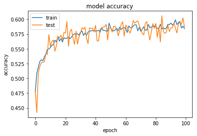
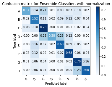
Increasing Performance with Ensembles

How do each of our preferred machine learning algorithms build their models? If they each have different strengths and weaknesses we may be able to build an ensemble model that outperforms the individual performance.

Looking at the Confusion Matrix for Insights

Luckily scikit-learn provides a helpful example that shows how to plot a confusion matrix. We will use this code below.

import itertools
import numpy as np
import matplotlib.pyplot as plt

from sklearn.model_selection import train_test_split
from sklearn.metrics import confusion_matrix

def plot_confusion_matrix(cm, classes,
                          normalize=False,
                          title='Confusion matrix',
                          cmap=plt.cm.Blues):
    """
    This function prints and plots the confusion matrix.
    Normalization can be applied by setting `normalize=True`.
    """
    if normalize:
        cm = cm.astype('float') / cm.sum(axis=1)[:, np.newaxis]
        print("Normalized confusion matrix")
    else:
        print('Confusion matrix, without normalization')

    print(cm)

    plt.imshow(cm, interpolation='nearest', cmap=cmap)
    plt.title(title)
    plt.colorbar()
    tick_marks = np.arange(len(classes))
    plt.xticks(tick_marks, classes, rotation=45)
    plt.yticks(tick_marks, classes)

    fmt = '.2f' if normalize else 'd'
    thresh = cm.max() / 2.
    for i, j in itertools.product(range(cm.shape[0]), range(cm.shape[1])):
        plt.text(j, i, format(cm[i, j], fmt),
                 horizontalalignment="center",
                 color="white" if cm[i, j] > thresh else "black")

    plt.tight_layout()
    plt.ylabel('True label')
    plt.xlabel('Predicted label')

# create the tokenizer
t = Tokenizer(num_words=5000)
# fit the tokenizer on the documents
t.fit_on_texts(docs)

X = t.texts_to_matrix(docs, mode="tfidf")

NBclf = MultinomialNB()
MLPclf = MLPClassifier()

X_train, X_test, y_train, y_test = train_test_split(X, Y_integers, random_state=0)

NB_y_pred = NBclf.fit(X_train, y_train).predict(X_test)
MLP_y_pred = MLPclf.fit(X_train, y_train).predict(X_test)

# Compute confusion matrix
NB_cnf_matrix = confusion_matrix(y_test, NB_y_pred)
MLP_cnf_matrix = confusion_matrix(y_test, MLP_y_pred)
np.set_printoptions(precision=2)

class_names = ['A', 'B', 'C', 'D', 'E', 'F', 'G', 'H']
# Plot non-normalized confusion matrix
plt.figure()
plot_confusion_matrix(NB_cnf_matrix, classes=class_names, normalize=True,
                      title='Confusion matrix for Naive Bayes, with normalization')

plt.figure()
plot_confusion_matrix(MLP_cnf_matrix, classes=class_names, normalize=True,
                      title='Confusion matrix for MLP Classifier, with normalization')

plt.show()

Normalized confusion matrix
[[0.34 0.14 0.22 0.01 0.11 0.07 0.1  0.01]
 [0.02 0.52 0.11 0.03 0.09 0.13 0.07 0.03]
 [0.08 0.1  0.73 0.   0.01 0.02 0.02 0.04]
 [0.   0.   0.25 0.38 0.25 0.12 0.   0.  ]
 [0.   0.14 0.07 0.02 0.62 0.09 0.05 0.02]
 [0.01 0.12 0.02 0.01 0.08 0.69 0.05 0.03]
 [0.01 0.06 0.04 0.   0.01 0.03 0.7  0.16]
 [0.   0.07 0.05 0.01 0.02 0.05 0.23 0.58]]
Normalized confusion matrix
[[0.63 0.1  0.1  0.   0.   0.03 0.07 0.05]
 [0.09 0.53 0.07 0.01 0.02 0.07 0.11 0.11]
 [0.25 0.12 0.48 0.   0.01 0.01 0.04 0.08]
 [0.25 0.25 0.25 0.   0.12 0.   0.   0.12]
 [0.16 0.19 0.03 0.   0.38 0.12 0.07 0.05]
 [0.12 0.17 0.01 0.   0.01 0.48 0.11 0.11]
 [0.04 0.03 0.02 0.   0.   0.02 0.67 0.21]
 [0.02 0.04 0.02 0.   0.   0.02 0.24 0.66]]

png

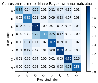
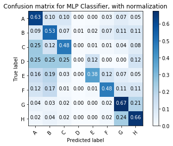
Observations on the Confusion Matrix

The Naive Bayes classifier performs better than the MLP classifier for Sections C, D, E, F and G. The MLP classifier performs better for Sections A, B, and H.

This suggests that an ensemble of both classifiers may work at improving performance. scikit-learn has a method to use both hard and soft voting here.

from sklearn.ensemble import VotingClassifier

estimators = []
estimators.append(('NB', NBclf))
estimators.append(('MLP', MLPclf))
# create the ensemble model
ensemble = VotingClassifier(estimators)
scores = cross_val_score(ensemble, X, Y_integers, cv=5)

scores

array([0.61, 0.59, 0.6 , 0.6 , 0.6 ])

scores.mean()*100

59.89522060313159

scores.std()*100

0.7295624868552363

# Trying soft voting
ensemble = VotingClassifier(estimators, voting = "soft")
scores = cross_val_score(ensemble, X, Y_integers, cv=5)

scores

array([0.61, 0.59, 0.6 , 0.6 , 0.6 ])

EN_y_pred = ensemble.fit(X_train, y_train).predict(X_test)

# Compute confusion matrix
EN_cnf_matrix = confusion_matrix(y_test, EN_y_pred)
np.set_printoptions(precision=2)

class_names = ['A', 'B', 'C', 'D', 'E', 'F', 'G', 'H']
# Plot non-normalized confusion matrix
plt.figure()
plot_confusion_matrix(EN_cnf_matrix, classes=class_names, normalize=True,
                      title='Confusion matrix for Ensemble Classifier, with normalization')

plt.show()

Normalized confusion matrix
[[0.37 0.14 0.21 0.01 0.09 0.07 0.1  0.02]
 [0.02 0.52 0.11 0.02 0.09 0.12 0.07 0.04]
 [0.08 0.1  0.73 0.   0.01 0.01 0.02 0.04]
 [0.   0.   0.25 0.38 0.25 0.12 0.   0.  ]
 [0.   0.16 0.07 0.02 0.6  0.09 0.05 0.02]
 [0.02 0.12 0.02 0.01 0.07 0.68 0.06 0.04]
 [0.01 0.06 0.04 0.   0.01 0.02 0.7  0.16]
 [0.   0.06 0.04 0.   0.01 0.05 0.23 0.6 ]]

png